View Jupyter notebook on the GitHub.
AutoML#
![]()
This notebooks covers AutoML utilities of ETNA library.
Hyperparameters tuning
How ``Tune` works <#section_1_1>`__
Example
General AutoML
How ``Auto` works <#section_2_1>`__
Example
[1]:
import warnings


warnings.filterwarnings("ignore")
[2]:
HORIZON = 14
Many features from this notebook require auto extension. You can install it by the command:
pip install etna[auto]
1. Hyperparameters tuning#
It is a common task to tune hyperparameters of existing pipeline to improve its quality. For this purpose there is an etna.auto.Tune class, which is responsible for creating optuna study to solve this problem.
In the next sections we will see how it works and how to use it for your particular problems.
1.1 How Tune works#
During init Tune accepts pipeline, its tuning parameters (params_to_tune), optimization metric (target_metric), parameters of backtest and parameters of optuna study.
In fit the optuna study is created. During each trial the sample of parameters is generated from params_to_tune and applied to pipeline. After that, the new pipeline is checked in backtest and target metric is returned to optuna framework.
Let’s look closer at params_to_tune parameter. It expects dictionary with parameter names and its distributions. But how this parameter names should be chosen?
1.1.1 set_params#
We are going to make a little detour to explain the set_params method, which is supported by ETNA pipelines, models and transforms. Given a dictionary with parameters it allows to create from existing object a new one with changed parameters.
First, we define some objects for our future examples.
[3]:
from etna.pipeline import Pipeline
from etna.models import LinearPerSegmentModel
from etna.transforms import LagTransform
from etna.transforms import DateFlagsTransform


model = LinearPerSegmentModel()
transforms = [
    LagTransform(in_column="target", lags=list(range(HORIZON, HORIZON + 10)), out_column="target_lag"),
    DateFlagsTransform(out_column="date_flags"),
]
pipeline = Pipeline(model=model, transforms=transforms, horizon=HORIZON)
Let’s look at simple example, when we want to change fit_intercept parameter of the model.
[4]:
model.to_dict()
[4]:
{'fit_intercept': True,
 'kwargs': {},
 '_target_': 'etna.models.linear.LinearPerSegmentModel'}
[5]:
new_model_params = {"fit_intercept": False}
new_model = model.set_params(**new_model_params)
new_model.to_dict()
[5]:
{'fit_intercept': False,
 'kwargs': {},
 '_target_': 'etna.models.linear.LinearPerSegmentModel'}
Great! On the next step we want to change the fit_intercept of model inside the pipeline.
[6]:
pipeline.to_dict()
[6]:
{'model': {'fit_intercept': True,
  'kwargs': {},
  '_target_': 'etna.models.linear.LinearPerSegmentModel'},
 'transforms': [{'in_column': 'target',
   'lags': [14, 15, 16, 17, 18, 19, 20, 21, 22, 23],
   'out_column': 'target_lag',
   '_target_': 'etna.transforms.math.lags.LagTransform'},
  {'day_number_in_week': True,
   'day_number_in_month': True,
   'day_number_in_year': False,
   'week_number_in_month': False,
   'week_number_in_year': False,
   'month_number_in_year': False,
   'season_number': False,
   'year_number': False,
   'is_weekend': True,
   'special_days_in_week': (),
   'special_days_in_month': (),
   'out_column': 'date_flags',
   '_target_': 'etna.transforms.timestamp.date_flags.DateFlagsTransform'}],
 'horizon': 14,
 '_target_': 'etna.pipeline.pipeline.Pipeline'}
[7]:
new_pipeline_params = {"model.fit_intercept": False}
new_pipeline = pipeline.set_params(**new_pipeline_params)
new_pipeline.to_dict()
[7]:
{'model': {'fit_intercept': False,
  'kwargs': {},
  '_target_': 'etna.models.linear.LinearPerSegmentModel'},
 'transforms': [{'in_column': 'target',
   'lags': [14, 15, 16, 17, 18, 19, 20, 21, 22, 23],
   'out_column': 'target_lag',
   '_target_': 'etna.transforms.math.lags.LagTransform'},
  {'day_number_in_week': True,
   'day_number_in_month': True,
   'day_number_in_year': False,
   'week_number_in_month': False,
   'week_number_in_year': False,
   'month_number_in_year': False,
   'season_number': False,
   'year_number': False,
   'is_weekend': True,
   'special_days_in_week': (),
   'special_days_in_month': (),
   'out_column': 'date_flags',
   '_target_': 'etna.transforms.timestamp.date_flags.DateFlagsTransform'}],
 'horizon': 14,
 '_target_': 'etna.pipeline.pipeline.Pipeline'}
Ok, it looks like we managed to do this. On the last step we are going to change is_weekend flag of DateFlagsTransform inside our pipeline.
[8]:
new_pipeline_params = {"transforms.1.is_weekend": False}
new_pipeline = pipeline.set_params(**new_pipeline_params)
new_pipeline.to_dict()
[8]:
{'model': {'fit_intercept': True,
  'kwargs': {},
  '_target_': 'etna.models.linear.LinearPerSegmentModel'},
 'transforms': [{'in_column': 'target',
   'lags': [14, 15, 16, 17, 18, 19, 20, 21, 22, 23],
   'out_column': 'target_lag',
   '_target_': 'etna.transforms.math.lags.LagTransform'},
  {'day_number_in_week': True,
   'day_number_in_month': True,
   'day_number_in_year': False,
   'week_number_in_month': False,
   'week_number_in_year': False,
   'month_number_in_year': False,
   'season_number': False,
   'year_number': False,
   'is_weekend': False,
   'special_days_in_week': (),
   'special_days_in_month': (),
   'out_column': 'date_flags',
   '_target_': 'etna.transforms.timestamp.date_flags.DateFlagsTransform'}],
 'horizon': 14,
 '_target_': 'etna.pipeline.pipeline.Pipeline'}
As we can see, we managed to do this.
1.1.2 params_to_tune#
Let’s get back to our initial question about params_to_tune. In our optuna study we are going to sample each parameter value from its distribution and pass it into pipeline.set_params method. So, the keys for params_to_tune should be a valid for set_params method.
Distributions are taken from etna.distributions and they are matching optuna.Trial.suggest_ methods.
For example, something like this will be valid for our pipeline defined above:
[9]:
from etna.distributions import CategoricalDistribution


example_params_to_tune = {
    "model.fit_intercept": CategoricalDistribution([False, True]),
    "transforms.0.is_weekend": CategoricalDistribution([False, True]),
}
There are some good news: it isn’t necessary for our users to define params_to_tune, because we have a default grid for many of our classes. The default grid is available by calling params_to_tune method on pipeline, model or transform. Let’s check our pipeline:
[10]:
pipeline.params_to_tune()
[10]:
{'model.fit_intercept': CategoricalDistribution(choices=[False, True]),
 'transforms.1.day_number_in_week': CategoricalDistribution(choices=[False, True]),
 'transforms.1.day_number_in_month': CategoricalDistribution(choices=[False, True]),
 'transforms.1.day_number_in_year': CategoricalDistribution(choices=[False, True]),
 'transforms.1.week_number_in_month': CategoricalDistribution(choices=[False, True]),
 'transforms.1.week_number_in_year': CategoricalDistribution(choices=[False, True]),
 'transforms.1.month_number_in_year': CategoricalDistribution(choices=[False, True]),
 'transforms.1.season_number': CategoricalDistribution(choices=[False, True]),
 'transforms.1.year_number': CategoricalDistribution(choices=[False, True]),
 'transforms.1.is_weekend': CategoricalDistribution(choices=[False, True])}
Now we are ready to use it in practice.
1.2 Example#
1.2.1 Loading data#
Let’s start by loading example data.
[11]:
import pandas as pd

from etna.datasets import TSDataset
[12]:
df = pd.read_csv("data/example_dataset.csv")
df.head()
[12]:
| timestamp | segment | target | |
|---|---|---|---|
| 0 | 2019-01-01 | segment_a | 170 |
| 1 | 2019-01-02 | segment_a | 243 |
| 2 | 2019-01-03 | segment_a | 267 |
| 3 | 2019-01-04 | segment_a | 287 |
| 4 | 2019-01-05 | segment_a | 279 |
[13]:
from etna.datasets import TSDataset

df = TSDataset.to_dataset(df)
full_ts = TSDataset(df, freq="D")
full_ts.plot()
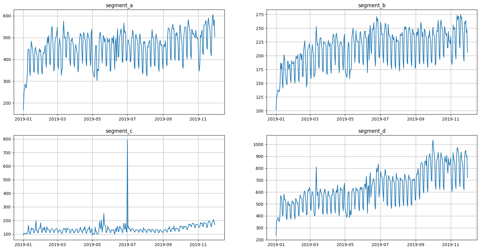
Let’s divide current dataset into train and validation parts. We will use validation part later to check final results.
[14]:
ts, _ = full_ts.train_test_split(test_size=HORIZON * 5)
1.2.2 Running Tune#
We are going to define our Tune object:
[15]:
from etna.metrics import SMAPE
from etna.auto import Tune


tune = Tune(pipeline=pipeline, target_metric=SMAPE(), horizon=HORIZON, backtest_params=dict(n_folds=5))
We used mostly default parameters for this example. But for your own experiments you might want to also set up other parameters.
For example, parameter runner allows you to run tuning in parallel on a local machine, and parameter storage makes it possible to store optuna results on a dedicated remote server.
For a full list of parameters we advise you to check our documentation.
Let’s hide the logs of optuna, there are too many of them for a notebook.
[16]:
import optuna


optuna.logging.set_verbosity(optuna.logging.CRITICAL)
Let’s run the tuning
[17]:
%%capture
best_pipeline = tune.fit(ts=ts, n_trials=20)
Command %%capture just hides the output.
1.2.3 Analysis#
In the last section dedicated to Tune we will look at methods for result analysis.
First of all there is summary method that shows us the results of optuna trials.
[18]:
tune.summary()
[18]:
| pipeline | hash | Sign_median | Sign_mean | Sign_std | Sign_percentile_5 | Sign_percentile_25 | Sign_percentile_75 | Sign_percentile_95 | SMAPE_median | ... | MSE_percentile_75 | MSE_percentile_95 | MedAE_median | MedAE_mean | MedAE_std | MedAE_percentile_5 | MedAE_percentile_25 | MedAE_percentile_75 | MedAE_percentile_95 | state | |
|---|---|---|---|---|---|---|---|---|---|---|---|---|---|---|---|---|---|---|---|---|---|
| 0 | Pipeline(model = LinearPerSegmentModel(fit_int... | f4f02e1d5f60b8f322a4a8a622dd1c1e | -0.500000 | -0.478571 | 0.205204 | -0.672857 | -0.621429 | -0.357143 | -0.254286 | 5.806429 | ... | 2220.282484 | 2953.865443 | 21.000232 | 22.334611 | 8.070926 | 14.955846 | 18.861388 | 24.473455 | 31.581505 | TrialState.COMPLETE |
| 1 | Pipeline(model = LinearPerSegmentModel(fit_int... | 3d7b7af16d71a36f3b935f69e113e22d | -0.457143 | -0.485714 | 0.242437 | -0.745714 | -0.642857 | -0.300000 | -0.265714 | 5.856039 | ... | 2644.982216 | 3294.855806 | 22.762122 | 23.389796 | 8.482028 | 14.897792 | 19.344439 | 26.807479 | 32.760543 | TrialState.COMPLETE |
| 2 | Pipeline(model = LinearPerSegmentModel(fit_int... | 7c7932114268832a5458acfecfb453fc | -0.200000 | -0.271429 | 0.264447 | -0.581429 | -0.392857 | -0.078571 | -0.061429 | 5.693983 | ... | 3457.757162 | 4209.624737 | 22.572681 | 23.336111 | 12.049564 | 11.235277 | 18.503043 | 27.405750 | 36.505748 | TrialState.COMPLETE |
| 3 | Pipeline(model = LinearPerSegmentModel(fit_int... | b7ac5f7fcf9c8959626befe263a9d561 | 0.000000 | -0.085714 | 0.211248 | -0.340000 | -0.100000 | 0.014286 | 0.048571 | 7.881275 | ... | 5039.841145 | 5665.228696 | 35.976862 | 33.937644 | 17.252826 | 14.444379 | 27.282228 | 42.632278 | 50.576005 | TrialState.COMPLETE |
| 4 | Pipeline(model = LinearPerSegmentModel(fit_int... | e928929f89156d88ef49e28abaf55847 | -0.414286 | -0.421429 | 0.207840 | -0.620000 | -0.585714 | -0.250000 | -0.232857 | 6.032319 | ... | 3091.962427 | 3181.592755 | 23.166650 | 25.265089 | 13.224461 | 13.001779 | 18.666844 | 29.764896 | 40.466215 | TrialState.COMPLETE |
| 5 | Pipeline(model = LinearPerSegmentModel(fit_int... | 3b4311d41fcaab7307235ea23b6d4599 | -0.400000 | -0.385714 | 0.396927 | -0.788571 | -0.514286 | -0.271429 | 0.037143 | 6.653462 | ... | 3800.976318 | 4837.444681 | 35.792514 | 32.276030 | 16.296588 | 13.499409 | 24.106508 | 43.962035 | 46.129572 | TrialState.COMPLETE |
| 6 | Pipeline(model = LinearPerSegmentModel(fit_int... | 74065ebc11c81bed6a9819d026c7cd84 | -0.442857 | -0.435714 | 0.246196 | -0.672857 | -0.621429 | -0.257143 | -0.188571 | 5.739626 | ... | 2933.246064 | 4802.299660 | 27.304852 | 24.936077 | 8.294963 | 15.108636 | 21.478207 | 30.762723 | 31.447233 | TrialState.COMPLETE |
| 7 | Pipeline(model = LinearPerSegmentModel(fit_int... | b0d0420255c6117045f8254bf8f377a0 | -0.442857 | -0.464286 | 0.260167 | -0.725714 | -0.657143 | -0.250000 | -0.232857 | 6.042134 | ... | 2682.735922 | 3688.168155 | 28.393903 | 25.819143 | 8.652993 | 15.618131 | 21.989342 | 32.223704 | 32.415490 | TrialState.COMPLETE |
| 8 | Pipeline(model = LinearPerSegmentModel(fit_int... | 25dcd8bb095f87a1ffc499fa6a83ef5d | -0.457143 | -0.457143 | 0.265986 | -0.705714 | -0.671429 | -0.242857 | -0.208571 | 5.869280 | ... | 3098.567787 | 3154.538337 | 22.380642 | 24.289797 | 11.998603 | 13.252341 | 19.168974 | 27.501465 | 38.000072 | TrialState.COMPLETE |
| 9 | Pipeline(model = LinearPerSegmentModel(fit_int... | 3f1ca1759261598081fa3bb2f32fe0ac | -0.414286 | -0.435714 | 0.292654 | -0.725714 | -0.657143 | -0.192857 | -0.175714 | 6.608191 | ... | 3044.388978 | 3611.477391 | 23.750327 | 26.488927 | 13.825791 | 14.242057 | 20.027917 | 30.211337 | 42.569838 | TrialState.COMPLETE |
| 10 | Pipeline(model = LinearPerSegmentModel(fit_int... | 8363309e454e72993f86f10c7fc7c137 | -0.157143 | -0.185714 | 0.226779 | -0.431429 | -0.328571 | -0.014286 | 0.020000 | 5.974832 | ... | 2902.306123 | 3526.513999 | 17.027383 | 21.682156 | 15.988286 | 9.110958 | 11.100846 | 27.608693 | 40.770037 | TrialState.COMPLETE |
| 11 | Pipeline(model = LinearPerSegmentModel(fit_int... | 8363309e454e72993f86f10c7fc7c137 | -0.157143 | -0.185714 | 0.226779 | -0.431429 | -0.328571 | -0.014286 | 0.020000 | 5.974832 | ... | 2902.306123 | 3526.513999 | 17.027383 | 21.682156 | 15.988286 | 9.110958 | 11.100846 | 27.608693 | 40.770037 | TrialState.COMPLETE |
| 12 | Pipeline(model = LinearPerSegmentModel(fit_int... | 8363309e454e72993f86f10c7fc7c137 | -0.157143 | -0.185714 | 0.226779 | -0.431429 | -0.328571 | -0.014286 | 0.020000 | 5.974832 | ... | 2902.306123 | 3526.513999 | 17.027383 | 21.682156 | 15.988286 | 9.110958 | 11.100846 | 27.608693 | 40.770037 | TrialState.COMPLETE |
| 13 | Pipeline(model = LinearPerSegmentModel(fit_int... | 8363309e454e72993f86f10c7fc7c137 | -0.157143 | -0.185714 | 0.226779 | -0.431429 | -0.328571 | -0.014286 | 0.020000 | 5.974832 | ... | 2902.306123 | 3526.513999 | 17.027383 | 21.682156 | 15.988286 | 9.110958 | 11.100846 | 27.608693 | 40.770037 | TrialState.COMPLETE |
| 14 | Pipeline(model = LinearPerSegmentModel(fit_int... | 8363309e454e72993f86f10c7fc7c137 | -0.157143 | -0.185714 | 0.226779 | -0.431429 | -0.328571 | -0.014286 | 0.020000 | 5.974832 | ... | 2902.306123 | 3526.513999 | 17.027383 | 21.682156 | 15.988286 | 9.110958 | 11.100846 | 27.608693 | 40.770037 | TrialState.COMPLETE |
| 15 | Pipeline(model = LinearPerSegmentModel(fit_int... | 8363309e454e72993f86f10c7fc7c137 | -0.157143 | -0.185714 | 0.226779 | -0.431429 | -0.328571 | -0.014286 | 0.020000 | 5.974832 | ... | 2902.306123 | 3526.513999 | 17.027383 | 21.682156 | 15.988286 | 9.110958 | 11.100846 | 27.608693 | 40.770037 | TrialState.COMPLETE |
| 16 | Pipeline(model = LinearPerSegmentModel(fit_int... | 8363309e454e72993f86f10c7fc7c137 | -0.157143 | -0.185714 | 0.226779 | -0.431429 | -0.328571 | -0.014286 | 0.020000 | 5.974832 | ... | 2902.306123 | 3526.513999 | 17.027383 | 21.682156 | 15.988286 | 9.110958 | 11.100846 | 27.608693 | 40.770037 | TrialState.COMPLETE |
| 17 | Pipeline(model = LinearPerSegmentModel(fit_int... | 8363309e454e72993f86f10c7fc7c137 | -0.157143 | -0.185714 | 0.226779 | -0.431429 | -0.328571 | -0.014286 | 0.020000 | 5.974832 | ... | 2902.306123 | 3526.513999 | 17.027383 | 21.682156 | 15.988286 | 9.110958 | 11.100846 | 27.608693 | 40.770037 | TrialState.COMPLETE |
| 18 | Pipeline(model = LinearPerSegmentModel(fit_int... | 6f595f4f43b323804c04d4cea49c169b | -0.414286 | -0.435714 | 0.325242 | -0.754286 | -0.685714 | -0.164286 | -0.147143 | 5.657316 | ... | 2247.347025 | 2681.501259 | 21.624614 | 22.111993 | 7.952462 | 14.197890 | 17.080865 | 26.655742 | 30.708428 | TrialState.COMPLETE |
| 19 | Pipeline(model = LinearPerSegmentModel(fit_int... | 8363309e454e72993f86f10c7fc7c137 | -0.157143 | -0.185714 | 0.226779 | -0.431429 | -0.328571 | -0.014286 | 0.020000 | 5.974832 | ... | 2902.306123 | 3526.513999 | 17.027383 | 21.682156 | 15.988286 | 9.110958 | 11.100846 | 27.608693 | 40.770037 | TrialState.COMPLETE |
20 rows × 38 columns
Let’s show only the columns we are interested in.
[19]:
tune.summary()[["hash", "pipeline", "SMAPE_mean", "state"]].sort_values("SMAPE_mean")
[19]:
| hash | pipeline | SMAPE_mean | state | |
|---|---|---|---|---|
| 19 | 8363309e454e72993f86f10c7fc7c137 | Pipeline(model = LinearPerSegmentModel(fit_int... | 8.556535 | TrialState.COMPLETE |
| 17 | 8363309e454e72993f86f10c7fc7c137 | Pipeline(model = LinearPerSegmentModel(fit_int... | 8.556535 | TrialState.COMPLETE |
| 16 | 8363309e454e72993f86f10c7fc7c137 | Pipeline(model = LinearPerSegmentModel(fit_int... | 8.556535 | TrialState.COMPLETE |
| 15 | 8363309e454e72993f86f10c7fc7c137 | Pipeline(model = LinearPerSegmentModel(fit_int... | 8.556535 | TrialState.COMPLETE |
| 14 | 8363309e454e72993f86f10c7fc7c137 | Pipeline(model = LinearPerSegmentModel(fit_int... | 8.556535 | TrialState.COMPLETE |
| 13 | 8363309e454e72993f86f10c7fc7c137 | Pipeline(model = LinearPerSegmentModel(fit_int... | 8.556535 | TrialState.COMPLETE |
| 12 | 8363309e454e72993f86f10c7fc7c137 | Pipeline(model = LinearPerSegmentModel(fit_int... | 8.556535 | TrialState.COMPLETE |
| 10 | 8363309e454e72993f86f10c7fc7c137 | Pipeline(model = LinearPerSegmentModel(fit_int... | 8.556535 | TrialState.COMPLETE |
| 11 | 8363309e454e72993f86f10c7fc7c137 | Pipeline(model = LinearPerSegmentModel(fit_int... | 8.556535 | TrialState.COMPLETE |
| 2 | 7c7932114268832a5458acfecfb453fc | Pipeline(model = LinearPerSegmentModel(fit_int... | 9.210183 | TrialState.COMPLETE |
| 8 | 25dcd8bb095f87a1ffc499fa6a83ef5d | Pipeline(model = LinearPerSegmentModel(fit_int... | 9.943658 | TrialState.COMPLETE |
| 4 | e928929f89156d88ef49e28abaf55847 | Pipeline(model = LinearPerSegmentModel(fit_int... | 9.946866 | TrialState.COMPLETE |
| 0 | f4f02e1d5f60b8f322a4a8a622dd1c1e | Pipeline(model = LinearPerSegmentModel(fit_int... | 9.957781 | TrialState.COMPLETE |
| 18 | 6f595f4f43b323804c04d4cea49c169b | Pipeline(model = LinearPerSegmentModel(fit_int... | 10.061742 | TrialState.COMPLETE |
| 1 | 3d7b7af16d71a36f3b935f69e113e22d | Pipeline(model = LinearPerSegmentModel(fit_int... | 10.306909 | TrialState.COMPLETE |
| 9 | 3f1ca1759261598081fa3bb2f32fe0ac | Pipeline(model = LinearPerSegmentModel(fit_int... | 10.554444 | TrialState.COMPLETE |
| 5 | 3b4311d41fcaab7307235ea23b6d4599 | Pipeline(model = LinearPerSegmentModel(fit_int... | 10.756703 | TrialState.COMPLETE |
| 6 | 74065ebc11c81bed6a9819d026c7cd84 | Pipeline(model = LinearPerSegmentModel(fit_int... | 10.917164 | TrialState.COMPLETE |
| 3 | b7ac5f7fcf9c8959626befe263a9d561 | Pipeline(model = LinearPerSegmentModel(fit_int... | 11.255320 | TrialState.COMPLETE |
| 7 | b0d0420255c6117045f8254bf8f377a0 | Pipeline(model = LinearPerSegmentModel(fit_int... | 11.478760 | TrialState.COMPLETE |
As we can see, we have duplicate lines according to the hash column. Some trials have the same sampled hyperparameters and they have the same results. We have a special handling for such duplicates: they are skipped during optimization and the previously computed metric values are returned.
Duplicates on the summary can be eliminated using hash column.
[20]:
tune.summary()[["hash", "pipeline", "SMAPE_mean", "state"]].sort_values("SMAPE_mean").drop_duplicates(subset="hash")
[20]:
| hash | pipeline | SMAPE_mean | state | |
|---|---|---|---|---|
| 19 | 8363309e454e72993f86f10c7fc7c137 | Pipeline(model = LinearPerSegmentModel(fit_int... | 8.556535 | TrialState.COMPLETE |
| 2 | 7c7932114268832a5458acfecfb453fc | Pipeline(model = LinearPerSegmentModel(fit_int... | 9.210183 | TrialState.COMPLETE |
| 8 | 25dcd8bb095f87a1ffc499fa6a83ef5d | Pipeline(model = LinearPerSegmentModel(fit_int... | 9.943658 | TrialState.COMPLETE |
| 4 | e928929f89156d88ef49e28abaf55847 | Pipeline(model = LinearPerSegmentModel(fit_int... | 9.946866 | TrialState.COMPLETE |
| 0 | f4f02e1d5f60b8f322a4a8a622dd1c1e | Pipeline(model = LinearPerSegmentModel(fit_int... | 9.957781 | TrialState.COMPLETE |
| 18 | 6f595f4f43b323804c04d4cea49c169b | Pipeline(model = LinearPerSegmentModel(fit_int... | 10.061742 | TrialState.COMPLETE |
| 1 | 3d7b7af16d71a36f3b935f69e113e22d | Pipeline(model = LinearPerSegmentModel(fit_int... | 10.306909 | TrialState.COMPLETE |
| 9 | 3f1ca1759261598081fa3bb2f32fe0ac | Pipeline(model = LinearPerSegmentModel(fit_int... | 10.554444 | TrialState.COMPLETE |
| 5 | 3b4311d41fcaab7307235ea23b6d4599 | Pipeline(model = LinearPerSegmentModel(fit_int... | 10.756703 | TrialState.COMPLETE |
| 6 | 74065ebc11c81bed6a9819d026c7cd84 | Pipeline(model = LinearPerSegmentModel(fit_int... | 10.917164 | TrialState.COMPLETE |
| 3 | b7ac5f7fcf9c8959626befe263a9d561 | Pipeline(model = LinearPerSegmentModel(fit_int... | 11.255320 | TrialState.COMPLETE |
| 7 | b0d0420255c6117045f8254bf8f377a0 | Pipeline(model = LinearPerSegmentModel(fit_int... | 11.478760 | TrialState.COMPLETE |
The second method top_k is useful when you want to check out best tried pipelines without duplicates.
[21]:
top_3_pipelines = tune.top_k(k=3)
[22]:
top_3_pipelines
[22]:
[Pipeline(model = LinearPerSegmentModel(fit_intercept = True, ), transforms = [LagTransform(in_column = 'target', lags = [14, 15, 16, 17, 18, 19, 20, 21, 22, 23], out_column = 'target_lag', ), DateFlagsTransform(day_number_in_week = False, day_number_in_month = True, day_number_in_year = False, week_number_in_month = True, week_number_in_year = False, month_number_in_year = False, season_number = False, year_number = False, is_weekend = True, special_days_in_week = (), special_days_in_month = (), out_column = 'date_flags', )], horizon = 14, ),
 Pipeline(model = LinearPerSegmentModel(fit_intercept = True, ), transforms = [LagTransform(in_column = 'target', lags = [14, 15, 16, 17, 18, 19, 20, 21, 22, 23], out_column = 'target_lag', ), DateFlagsTransform(day_number_in_week = False, day_number_in_month = True, day_number_in_year = False, week_number_in_month = True, week_number_in_year = False, month_number_in_year = False, season_number = False, year_number = False, is_weekend = False, special_days_in_week = (), special_days_in_month = (), out_column = 'date_flags', )], horizon = 14, ),
 Pipeline(model = LinearPerSegmentModel(fit_intercept = False, ), transforms = [LagTransform(in_column = 'target', lags = [14, 15, 16, 17, 18, 19, 20, 21, 22, 23], out_column = 'target_lag', ), DateFlagsTransform(day_number_in_week = True, day_number_in_month = False, day_number_in_year = True, week_number_in_month = False, week_number_in_year = False, month_number_in_year = False, season_number = False, year_number = True, is_weekend = False, special_days_in_week = (), special_days_in_month = (), out_column = 'date_flags', )], horizon = 14, )]
2. General AutoML#
Hyperparameters tuning is useful, but can be too narrow. In this section we move our attention to general AutoML pipeline. In ETNA we have an etna.auto.Auto class for making automatic pipeline selection. It can be useful to quickly create a good baseline for your forecasting task.
2.1 How Auto works#
Auto init has similar parameters to Tune, but instead of pipeline it works with pool. Pool, in general, is just a list of pipelines.
During fit there are two stages: - pool stage, - tuning stage.
Pool stage is responsible for checking every pipeline suggested in a given pool. For each pipeline we run a backtest and compute target_metric. Results are saved in optuna study.
Tuning stage takes tune_size best pipelines according to the resuls of the pool stage. And then runs Tune with default params_to_tune for them sequentially from best to the worst.
Limit parameters n_trials and timeout are shared between pool and tuning stages. First, we run pool stage with given n_trials and timeout. After that, the remaining values are divided equally among tune_size tuning steps.
2.2 Example#
We will move stright to the example.
[23]:
from etna.auto import Auto


auto = Auto(target_metric=SMAPE(), horizon=HORIZON, backtest_params=dict(n_folds=5))
We used mostly default parameters, even pool. There is also a default sampler, but to make results more reproducible we fixed the seed.
Let’s start the fitting. We can start by running only pool stage.
[24]:
%%capture
best_pool_pipeline = auto.fit(ts=ts, tune_size=0)
[25]:
auto.summary()[["hash", "pipeline", "SMAPE_mean", "state", "study"]].sort_values("SMAPE_mean")
[25]:
| hash | pipeline | SMAPE_mean | state | study | |
|---|---|---|---|---|---|
| 15 | af8088ac0abfde46e93a8dbb407a2117 | Pipeline(model = CatBoostPerSegmentModel(itera... | 5.057438 | TrialState.COMPLETE | pool |
| 2 | d8215d95e2c6c9a4b4fdacf3fa77dddc | Pipeline(model = NaiveModel(lag = 7, ), transf... | 5.164436 | TrialState.COMPLETE | pool |
| 14 | 8f640faabcac0552153ca19337179f3b | Pipeline(model = HoltWintersModel(trend = 'add... | 5.931951 | TrialState.COMPLETE | pool |
| 10 | d6a44adb551f1aec09ef37c14aed260f | Pipeline(model = SeasonalMovingAverageModel(wi... | 6.197182 | TrialState.COMPLETE | pool |
| 16 | 16eb77200eb2fd5dc1f6f2a5067884cd | Pipeline(model = HoltWintersModel(trend = 'add... | 6.347734 | TrialState.COMPLETE | pool |
| 13 | 4c07749e913403906cd033e4882fc4f9 | Pipeline(model = SeasonalMovingAverageModel(wi... | 6.529721 | TrialState.COMPLETE | pool |
| 5 | 6e2eb71d033b6d0607f5b6d0a7596ce9 | Pipeline(model = ProphetModel(growth = 'linear... | 7.799984 | TrialState.COMPLETE | pool |
| 17 | 6bb58e7ce09eab00448d5732240ec2ec | Pipeline(model = CatBoostMultiSegmentModel(ite... | 7.814187 | TrialState.COMPLETE | pool |
| 18 | a640ddfb767ea0cbf31751ddda6e36ee | Pipeline(model = CatBoostMultiSegmentModel(ite... | 7.816528 | TrialState.COMPLETE | pool |
| 9 | cfeb21bcf2e922a390ade8be9d845e0d | Pipeline(model = ProphetModel(growth = 'linear... | 7.893421 | TrialState.COMPLETE | pool |
| 3 | a5e036978ef9cc9f297c9eb2c280af05 | Pipeline(model = AutoARIMAModel(), transforms ... | 8.297048 | TrialState.COMPLETE | pool |
| 0 | 2e36e0b9cb67a43bb1bf96fa2ccf718f | Pipeline(model = LinearMultiSegmentModel(fit_i... | 9.205423 | TrialState.COMPLETE | pool |
| 4 | 8b9f5fa09754a80f17380dec2b998f1d | Pipeline(model = LinearPerSegmentModel(fit_int... | 10.997462 | TrialState.COMPLETE | pool |
| 1 | d62c0579459d4a1b88aea8ed6effdf4e | Pipeline(model = MovingAverageModel(window = 1... | 11.317256 | TrialState.COMPLETE | pool |
| 6 | 5916e5b653295271c79caae490618ee9 | Pipeline(model = MovingAverageModel(window = 2... | 12.028916 | TrialState.COMPLETE | pool |
| 11 | 5a91b6c8acc2c461913df44fd1429375 | Pipeline(model = ElasticPerSegmentModel(alpha ... | 12.213320 | TrialState.COMPLETE | pool |
| 7 | 403b3e18012af5ff9815b408f5c2e47d | Pipeline(model = MovingAverageModel(window = 4... | 12.243011 | TrialState.COMPLETE | pool |
| 19 | 6cf8605e6c513053ac4f5203e330c59d | Pipeline(model = HoltWintersModel(trend = None... | 15.473118 | TrialState.COMPLETE | pool |
| 12 | 53e90ae4cf7f1f71e6396107549c25ef | Pipeline(model = NaiveModel(lag = 1, ), transf... | 19.361078 | TrialState.COMPLETE | pool |
| 8 | 90b31b54cb8c01867be05a3320852682 | Pipeline(model = ElasticMultiSegmentModel(alph... | 35.971289 | TrialState.COMPLETE | pool |
We can continue our training. The pool stage is over and there will be only the tuning stage. If we don’t want to wait forever we should limit the tuning by fixing n_trials or timeout.
We also set some parameters for optuna.Study.optimize: - gc_after_trial=True: to prevent fit from increasing memory consumption - catch=(Exception,): to prevent failing if some trials are erroneous.
[26]:
%%capture
best_tuning_pipeline = auto.fit(ts=ts, tune_size=3, n_trials=100, gc_after_trial=True, catch=(Exception,))
Let’s look at the results.
[27]:
auto.summary()[["hash", "pipeline", "SMAPE_mean", "state", "study"]].sort_values("SMAPE_mean").drop_duplicates(
    subset=("hash", "study")
).head(10)
[27]:
| hash | pipeline | SMAPE_mean | state | study | |
|---|---|---|---|---|---|
| 56 | 419fc80cf634ba0888c4f899f666ad45 | Pipeline(model = HoltWintersModel(trend = 'mul... | 4.769471 | TrialState.COMPLETE | tuning/8f640faabcac0552153ca19337179f3b |
| 89 | 731ccb72a473bec81789b7f186001ddd | Pipeline(model = CatBoostPerSegmentModel(itera... | 4.899715 | TrialState.COMPLETE | tuning/af8088ac0abfde46e93a8dbb407a2117 |
| 97 | 9c302769456b4adb9143f11c582f7264 | Pipeline(model = CatBoostPerSegmentModel(itera... | 4.927197 | TrialState.COMPLETE | tuning/af8088ac0abfde46e93a8dbb407a2117 |
| 88 | 182c748af70287ab3a12bf32c03320f5 | Pipeline(model = CatBoostPerSegmentModel(itera... | 4.941247 | TrialState.COMPLETE | tuning/af8088ac0abfde46e93a8dbb407a2117 |
| 96 | 4f426335c0eb00d847d9dd1e0a421415 | Pipeline(model = CatBoostPerSegmentModel(itera... | 4.977773 | TrialState.COMPLETE | tuning/af8088ac0abfde46e93a8dbb407a2117 |
| 98 | 2cafd0750f191e7ab2d4160da50a7c64 | Pipeline(model = CatBoostPerSegmentModel(itera... | 5.056993 | TrialState.COMPLETE | tuning/af8088ac0abfde46e93a8dbb407a2117 |
| 15 | af8088ac0abfde46e93a8dbb407a2117 | Pipeline(model = CatBoostPerSegmentModel(itera... | 5.057438 | TrialState.COMPLETE | pool |
| 75 | 382825866425cac211691205a9537c95 | Pipeline(model = CatBoostPerSegmentModel(itera... | 5.081609 | TrialState.COMPLETE | tuning/af8088ac0abfde46e93a8dbb407a2117 |
| 95 | c2a8d498fe35873d060e173e1af042d5 | Pipeline(model = CatBoostPerSegmentModel(itera... | 5.117583 | TrialState.COMPLETE | tuning/af8088ac0abfde46e93a8dbb407a2117 |
| 91 | 035f8e28180bc7491a30b3d0d67060c9 | Pipeline(model = CatBoostPerSegmentModel(itera... | 5.135956 | TrialState.COMPLETE | tuning/af8088ac0abfde46e93a8dbb407a2117 |
[28]:
auto.top_k(k=5)
[28]:
[Pipeline(model = HoltWintersModel(trend = 'mul', damped_trend = False, seasonal = 'mul', seasonal_periods = None, initialization_method = 'estimated', initial_level = None, initial_trend = None, initial_seasonal = None, use_boxcox = True, bounds = None, dates = None, freq = None, missing = 'none', smoothing_level = None, smoothing_trend = None, smoothing_seasonal = None, damping_trend = None, ), transforms = [], horizon = 14, ),
 Pipeline(model = CatBoostPerSegmentModel(iterations = None, depth = 9, learning_rate = 0.0435214895575014, logging_level = 'Silent', l2_leaf_reg = 1.588756097852857, thread_count = None, random_strength = 0.0001602176189749599, ), transforms = [LagTransform(in_column = 'target', lags = [15, 16, 17, 18, 19, 20, 21, 22, 23, 24, 25, 26, 27, 28], out_column = None, ), DateFlagsTransform(day_number_in_week = True, day_number_in_month = False, day_number_in_year = False, week_number_in_month = False, week_number_in_year = False, month_number_in_year = False, season_number = False, year_number = False, is_weekend = True, special_days_in_week = [], special_days_in_month = [], out_column = None, )], horizon = 14, ),
 Pipeline(model = CatBoostPerSegmentModel(iterations = None, depth = 10, learning_rate = 0.066387199945575, logging_level = 'Silent', l2_leaf_reg = 3.8476771557403033, thread_count = None, random_strength = 2.6976801196146113e-05, ), transforms = [LagTransform(in_column = 'target', lags = [15, 16, 17, 18, 19, 20, 21, 22, 23, 24, 25, 26, 27, 28], out_column = None, ), DateFlagsTransform(day_number_in_week = True, day_number_in_month = False, day_number_in_year = False, week_number_in_month = False, week_number_in_year = False, month_number_in_year = False, season_number = False, year_number = False, is_weekend = True, special_days_in_week = [], special_days_in_month = [], out_column = None, )], horizon = 14, ),
 Pipeline(model = CatBoostPerSegmentModel(iterations = None, depth = 8, learning_rate = 0.1368955392889537, logging_level = 'Silent', l2_leaf_reg = 1.8121398100968207, thread_count = None, random_strength = 1.0292981436693363e-05, ), transforms = [LagTransform(in_column = 'target', lags = [15, 16, 17, 18, 19, 20, 21, 22, 23, 24, 25, 26, 27, 28], out_column = None, ), DateFlagsTransform(day_number_in_week = True, day_number_in_month = True, day_number_in_year = True, week_number_in_month = False, week_number_in_year = False, month_number_in_year = False, season_number = False, year_number = False, is_weekend = True, special_days_in_week = [], special_days_in_month = [], out_column = None, )], horizon = 14, ),
 Pipeline(model = CatBoostPerSegmentModel(iterations = None, depth = 10, learning_rate = 0.04930475651736648, logging_level = 'Silent', l2_leaf_reg = 1.2938317623739193, thread_count = None, random_strength = 0.00020141074677370956, ), transforms = [LagTransform(in_column = 'target', lags = [15, 16, 17, 18, 19, 20, 21, 22, 23, 24, 25, 26, 27, 28], out_column = None, ), DateFlagsTransform(day_number_in_week = True, day_number_in_month = False, day_number_in_year = False, week_number_in_month = False, week_number_in_year = False, month_number_in_year = False, season_number = False, year_number = False, is_weekend = True, special_days_in_week = [], special_days_in_month = [], out_column = None, )], horizon = 14, )]
If we look at study column we will see that best trial from tuning stage is better then best trial from pool stage. It means, that tuning stage was successful and improved the final result.
Let’s compare best pipeline on pool and tuning stages on hold-out part of initial ts.
[29]:
%%capture
best_pool_metrics, _, _ = best_pool_pipeline.backtest(ts=full_ts, metrics=[SMAPE()], n_folds=5)
best_tuning_metrics, _, _ = best_tuning_pipeline.backtest(ts=full_ts, metrics=[SMAPE()], n_folds=5)
[30]:
best_pool_smape = best_pool_metrics["SMAPE"].mean()
best_tuning_smape = best_tuning_metrics["SMAPE"].mean()
print(f"Best pool SMAPE: {best_pool_smape:.3f}")
print(f"Best tuning SMAPE: {best_tuning_smape:.3f}")
Best pool SMAPE: 8.262
Best tuning SMAPE: 8.188
As we can see, the results are slightly better after the tuning stage, but it can be statistically insignificant. For your datasets the results could be different.
3. Summary#
In this notebook we discussed how AutoML works in ETNA library and how to use it. There are two supported scenarios: - Tuning your existing pipeline; - Automatic search of the pipeline for your forecasting task.