View Jupyter notebook on the GitHub.
Regressors and exogenous data#
![]()
This notebook serves as a tutorial for:
Loading regressors to TSDataset
Training and using a model with regressors
Table of Contents
What is regressor?
What is exogenous data?
Dataset
Loading Dataset
EDA
Forecast with regressors
1. What is regressor?#
In previous tutorials, we have shown how to work with target time series.
Target time series is a time series we want to forecast.
But imagine that you have information about the future that can help model with forecasting target time series. It may be information about holidays, weather, recurring events, marketing campaigns, etc. We will call it regressor.
Regressor is a time series that we are not interested in forecasting, however, it may help to forecast the target time series.
To apply an ML model that uses regressors to make more accurate forecasts, we need to know how regressors affected the target time series in the past and information about their values in the future.
What is additional data?#
There is also data that we don’t know in advance. However using it still allows us to make more accurate forecasts. This data we will call additional data. For example, if many users bought a new phone few weeks ago we should expect more support requests on this product.
In order to use additional data in ML models we should create regressors out of them. For example, it could be done with LagTransform or TrendTransform.
In this tutorial we will not look at additional data and will focus on regressors.
2. Dataset#
ETNA allows working with regressor as convenient as with target time series.
We are going to forecast the time series from Tabular Playground Series - Jan 2022. The dataset contains daily merchandise sales – mugs, hats, and stickers – at two imaginary store chains across three Scandinavian countries. As exogenous data, we will use Finland, Norway, and Sweden Weather Data 2015-2019 dataset containing daily country average precipitation, snow depth and air temperature data.
2.1 Loading Dataset#
First, let’s load the data.
[1]:
import pandas as pd
import warnings

warnings.filterwarnings("ignore")

target_df = pd.read_csv("data/nordic_merch_sales.csv")
regressor_df = pd.read_csv("data/nordics_weather.csv")
The next step is converting the data into the ETNA format. Code that allows us to do that is identical for target time series and exogenous data.
[2]:
from etna.datasets import TSDataset

target_df = TSDataset.to_dataset(target_df)
target_df.tail()
[2]:
| segment | Finland_KaggleMart_Kaggle Hat | Finland_KaggleMart_Kaggle Mug | Finland_KaggleMart_Kaggle Sticker | Finland_KaggleRama_Kaggle Hat | Finland_KaggleRama_Kaggle Mug | Finland_KaggleRama_Kaggle Sticker | Norway_KaggleMart_Kaggle Hat | Norway_KaggleMart_Kaggle Mug | Norway_KaggleMart_Kaggle Sticker | Norway_KaggleRama_Kaggle Hat | Norway_KaggleRama_Kaggle Mug | Norway_KaggleRama_Kaggle Sticker | Sweden_KaggleMart_Kaggle Hat | Sweden_KaggleMart_Kaggle Mug | Sweden_KaggleMart_Kaggle Sticker | Sweden_KaggleRama_Kaggle Hat | Sweden_KaggleRama_Kaggle Mug | Sweden_KaggleRama_Kaggle Sticker |
|---|---|---|---|---|---|---|---|---|---|---|---|---|---|---|---|---|---|---|
| feature | target | target | target | target | target | target | target | target | target | target | target | target | target | target | target | target | target | target |
| timestamp | ||||||||||||||||||
| 2018-12-27 | 573 | 414 | 177 | 1068 | 652 | 308 | 898 | 568 | 270 | 1604 | 1108 | 436 | 672 | 420 | 196 | 1127 | 745 | 319 |
| 2018-12-28 | 841 | 499 | 223 | 1398 | 895 | 431 | 1162 | 731 | 361 | 2178 | 1333 | 662 | 874 | 555 | 260 | 1540 | 990 | 441 |
| 2018-12-29 | 1107 | 774 | 296 | 1895 | 1398 | 559 | 1650 | 1113 | 518 | 2884 | 1816 | 874 | 1106 | 720 | 348 | 2169 | 1438 | 596 |
| 2018-12-30 | 1113 | 757 | 326 | 1878 | 1241 | 554 | 1809 | 1052 | 500 | 2851 | 1935 | 833 | 1133 | 730 | 336 | 2138 | 1303 | 587 |
| 2018-12-31 | 822 | 469 | 238 | 1231 | 831 | 360 | 1124 | 728 | 351 | 2128 | 1383 | 561 | 823 | 570 | 250 | 1441 | 1004 | 388 |
As you can see, the target ends in 2018, and the exogenous data ends in 2019, so we have prior information a year ahead. This implies that our exogenous data contains only regressors.
[3]:
regressor_df = TSDataset.to_dataset(regressor_df)
regressor_df.tail()
[3]:
| segment | Finland_KaggleMart_Kaggle Hat | Finland_KaggleMart_Kaggle Mug | ... | Sweden_KaggleRama_Kaggle Mug | Sweden_KaggleRama_Kaggle Sticker | ||||||||||||||||
|---|---|---|---|---|---|---|---|---|---|---|---|---|---|---|---|---|---|---|---|---|---|
| feature | precipitation | snow_depth | tavg | tmax | tmin | precipitation | snow_depth | tavg | tmax | tmin | ... | precipitation | snow_depth | tavg | tmax | tmin | precipitation | snow_depth | tavg | tmax | tmin |
| timestamp | |||||||||||||||||||||
| 2019-12-27 | 0.028249 | 109.550000 | -8.529630 | -3.161039 | -10.895425 | 0.028249 | 109.550000 | -8.529630 | -3.161039 | -10.895425 | ... | 0.105079 | 141.220930 | -4.277778 | -2.391204 | -8.993458 | 0.105079 | 141.220930 | -4.277778 | -2.391204 | -8.993458 |
| 2019-12-28 | 0.789266 | 116.421053 | -9.107407 | -4.703947 | -15.288889 | 0.789266 | 116.421053 | -9.107407 | -4.703947 | -15.288889 | ... | 1.117688 | 142.955224 | -3.866667 | -3.006542 | -11.593056 | 1.117688 | 142.955224 | -3.866667 | -3.006542 | -11.593056 |
| 2019-12-29 | 4.976966 | 117.117647 | -0.418519 | 1.264052 | -7.722078 | 4.976966 | 117.117647 | -0.418519 | 1.264052 | -7.722078 | ... | 1.758669 | 136.725146 | 1.755556 | 3.692056 | -4.516204 | 1.758669 | 136.725146 | 1.755556 | 3.692056 | -4.516204 |
| 2019-12-30 | 1.229775 | 160.500000 | 2.292593 | 3.344156 | -0.202632 | 1.229775 | 160.500000 | 2.292593 | 3.344156 | -0.202632 | ... | 0.561996 | 120.740741 | 4.900000 | 6.135648 | 1.859070 | 0.561996 | 120.740741 | 4.900000 | 6.135648 | 1.859070 |
| 2019-12-31 | 0.225281 | 124.647059 | -2.859259 | 1.580519 | -6.921569 | 0.225281 | 124.647059 | -2.859259 | 1.580519 | -6.921569 | ... | 0.848161 | 131.583333 | 1.722222 | 4.376606 | -2.290278 | 0.848161 | 131.583333 | 1.722222 | 4.376606 | -2.290278 |
5 rows × 90 columns
Then we have to create TSDataset with both target time series and exogenous data. TSDataset expects us to put target time series in df argument and exogenous data in df_exog. We should do it because regressors contain information about the target’s future. TSDataset ensures we don’t mix them.
In order to specify the columns of df_exog, which contains regressors, we need to use the known_future parameter. This allows TSDataset to determine which columns are regressors and which columns are additional data.
[4]:
ts = TSDataset(df=target_df, freq="D", df_exog=regressor_df, known_future="all")
ts.head()
[4]:
| segment | Finland_KaggleMart_Kaggle Hat | Finland_KaggleMart_Kaggle Mug | ... | Sweden_KaggleRama_Kaggle Mug | Sweden_KaggleRama_Kaggle Sticker | ||||||||||||||||
|---|---|---|---|---|---|---|---|---|---|---|---|---|---|---|---|---|---|---|---|---|---|
| feature | precipitation | snow_depth | target | tavg | tmax | tmin | precipitation | snow_depth | target | tavg | ... | target | tavg | tmax | tmin | precipitation | snow_depth | target | tavg | tmax | tmin |
| timestamp | |||||||||||||||||||||
| 2015-01-01 | 1.714141 | 284.545455 | 520.0 | 1.428571 | 2.912739 | -1.015287 | 1.714141 | 284.545455 | 329.0 | 1.428571 | ... | 706.0 | 3.47 | 5.415354 | 0.221569 | 3.642278 | 84.924623 | 324.0 | 3.47 | 5.415354 | 0.221569 |
| 2015-01-02 | 10.016667 | 195.000000 | 493.0 | 0.553571 | 2.358599 | -0.998718 | 10.016667 | 195.000000 | 318.0 | 0.553571 | ... | 653.0 | 3.80 | 5.097244 | 0.294882 | 2.414665 | 67.043702 | 293.0 | 3.80 | 5.097244 | 0.294882 |
| 2015-01-03 | 3.956061 | 284.294118 | 535.0 | -1.739286 | 0.820382 | -3.463871 | 3.956061 | 284.294118 | 360.0 | -1.739286 | ... | 734.0 | 1.61 | 2.140392 | -1.776680 | 0.212793 | 79.945946 | 319.0 | 1.61 | 2.140392 | -1.776680 |
| 2015-01-04 | 0.246193 | 260.772727 | 544.0 | -7.035714 | -3.110828 | -9.502581 | 0.246193 | 260.772727 | 332.0 | -7.035714 | ... | 657.0 | -1.35 | -0.648425 | -5.173123 | 0.226833 | 78.997290 | 300.0 | -1.35 | -0.648425 | -5.173123 |
| 2015-01-05 | 0.036364 | 236.900000 | 378.0 | -17.164286 | -8.727564 | -19.004487 | 0.036364 | 236.900000 | 243.0 | -17.164286 | ... | 512.0 | -4.27 | -3.027451 | -9.544488 | 0.515601 | 79.736148 | 227.0 | -4.27 | -3.027451 | -9.544488 |
5 rows × 108 columns
2.2 EDA#
TSDataset joins exogenous data and the target time series, so we can visualize and analyze exogenous data in the same way as target time series. More information in EDA notebook.
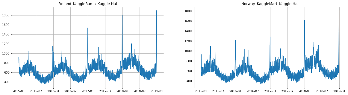
[5]:
ts.plot(column="snow_depth", n_segments=2)
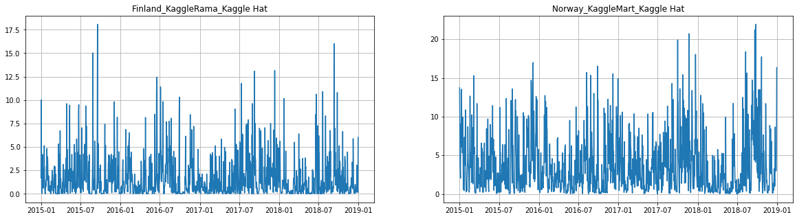
[6]:
ts.plot(column="precipitation", n_segments=2)
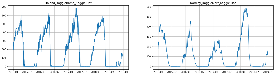
[7]:
ts.plot(column="target", n_segments=2)
3. Forecast with regressors#
We will use LinearPerSegmentModel. It is a simple model that works with regressors.
Note: some models do not work with regressors. In this case, they will warn you about it.
We should forecast merchandise sales a year ahead using regressors with information about weather.
[8]:
from etna.models import LinearPerSegmentModel

HORIZON = 365
model = LinearPerSegmentModel()
ETNA allows to configure the transforms to work with exogenous data the same way as they work with the time series. In addition to this, transforms will automatically update information about regressors in TSDataset.
[9]:
from etna.transforms import FilterFeaturesTransform

from etna.transforms import MeanTransform  # math
from etna.transforms import DateFlagsTransform, HolidayTransform  # datetime
from etna.transforms import LagTransform  # lags

transforms = [
    LagTransform(
        in_column="target",
        lags=list(range(HORIZON, HORIZON + 28)),
        out_column="target_lag",
    ),
    LagTransform(in_column="tavg", lags=list(range(1, 3)), out_column="tavg_lag"),
    MeanTransform(in_column="tavg", window=7, out_column="tavg_mean"),
    MeanTransform(
        in_column="target_lag_365",
        out_column="target_mean",
        window=104,
        seasonality=7,
    ),
    DateFlagsTransform(
        day_number_in_week=True,
        day_number_in_month=True,
        is_weekend=True,
        special_days_in_week=[4],
        out_column="date_flag",
    ),
    HolidayTransform(iso_code="SWE", out_column="SWE_holidays"),
    HolidayTransform(iso_code="NOR", out_column="NOR_holidays"),
    HolidayTransform(iso_code="FIN", out_column="FIN_holidays"),
    LagTransform(
        in_column="SWE_holidays",
        lags=list(range(2, 6)),
        out_column="SWE_holidays_lag",
    ),
    LagTransform(
        in_column="NOR_holidays",
        lags=list(range(2, 6)),
        out_column="NOR_holidays_lag",
    ),
    LagTransform(
        in_column="FIN_holidays",
        lags=list(range(2, 6)),
        out_column="FIN_holidays_lag",
    ),
    FilterFeaturesTransform(exclude=["precipitation", "snow_depth", "tmin", "tmax"]),
]
The next steps are literally identical to the situation when we work with target time series only.
[10]:
from etna.pipeline import Pipeline

pipeline = Pipeline(model=model, transforms=transforms, horizon=HORIZON)
[11]:
from etna.metrics import SMAPE

metrics, forecasts, _ = pipeline.backtest(ts, metrics=[SMAPE()], aggregate_metrics=True, n_folds=2)
[Parallel(n_jobs=1)]: Using backend SequentialBackend with 1 concurrent workers.
[Parallel(n_jobs=1)]: Done   1 out of   1 | elapsed:    3.2s remaining:    0.0s
[Parallel(n_jobs=1)]: Done   2 out of   2 | elapsed:    6.5s remaining:    0.0s
[Parallel(n_jobs=1)]: Done   2 out of   2 | elapsed:    6.5s finished
[12]:
metrics
[12]:
| segment | SMAPE | |
|---|---|---|
| 0 | Finland_KaggleMart_Kaggle Hat | 6.809976 |
| 1 | Finland_KaggleMart_Kaggle Mug | 7.897876 |
| 2 | Finland_KaggleMart_Kaggle Sticker | 7.566816 |
| 3 | Finland_KaggleRama_Kaggle Hat | 6.714908 |
| 4 | Finland_KaggleRama_Kaggle Mug | 7.443409 |
| 5 | Finland_KaggleRama_Kaggle Sticker | 7.540571 |
| 6 | Norway_KaggleMart_Kaggle Hat | 9.335215 |
| 7 | Norway_KaggleMart_Kaggle Mug | 11.929340 |
| 8 | Norway_KaggleMart_Kaggle Sticker | 11.455042 |
| 9 | Norway_KaggleRama_Kaggle Hat | 8.976252 |
| 10 | Norway_KaggleRama_Kaggle Mug | 11.691445 |
| 11 | Norway_KaggleRama_Kaggle Sticker | 11.594758 |
| 12 | Sweden_KaggleMart_Kaggle Hat | 6.837174 |
| 13 | Sweden_KaggleMart_Kaggle Mug | 7.319936 |
| 14 | Sweden_KaggleMart_Kaggle Sticker | 6.973164 |
| 15 | Sweden_KaggleRama_Kaggle Hat | 6.366672 |
| 16 | Sweden_KaggleRama_Kaggle Mug | 6.994042 |
| 17 | Sweden_KaggleRama_Kaggle Sticker | 7.081337 |
[13]:
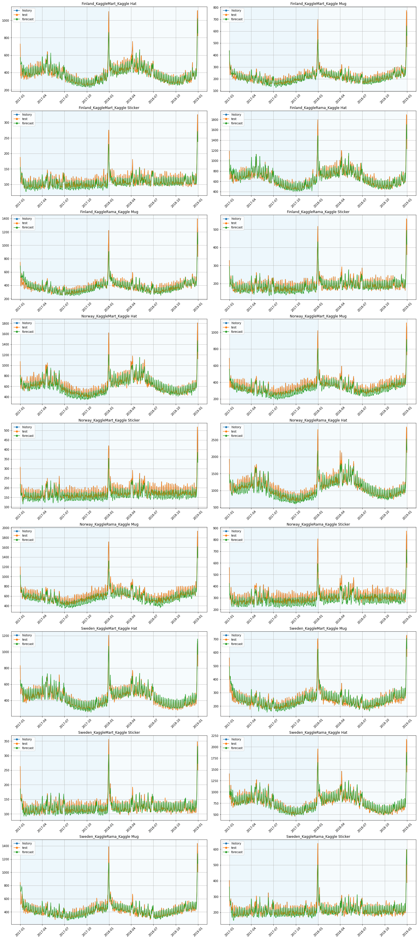
from etna.analysis import plot_backtest

plot_backtest(forecasts, ts)
Supporting more work strategies for regressors and additional data is a future feature on the ETNA development roadmap.