View Jupyter notebook on the GitHub.
Forecasting strategies#
There are 5 possible forecasting strategies:
Recursive: sequentially forecasts
steppoints and use them to forecast next points.Direct: uses separate model to forecast each time subsegment
DirRec: uses a separate model to forecast each time subsegment, fitting the next model on the train set extended with the forecasts of previous models
MIMO: uses a single multi-output model
DIRMO: MIMO + DirREC
The first two of these strategies are available in ETNA, and we will take a closer look at them in this notebook.
Notebook navigation: * Imports and constants * Load dataset * Recursive strategy * AutoRegressivePipeline * Direct strategy * Pipeline * DirectEnsemble * assemble_pipelines + DirectEnsemble * Summary
0. Imports and constants#
[1]:
import warnings

warnings.filterwarnings("ignore")
[2]:
import pandas as pd
from etna.datasets import TSDataset
from etna.models import CatBoostPerSegmentModel
from etna.transforms import LagTransform
from etna.transforms import LinearTrendTransform
from etna.metrics import SMAPE, MAE, MAPE
from etna.analysis import plot_backtest

HORIZON = 14
HISTORY_LEN = 5 * HORIZON
NUMBER_OF_LAGS = 21
1. Load Dataset#
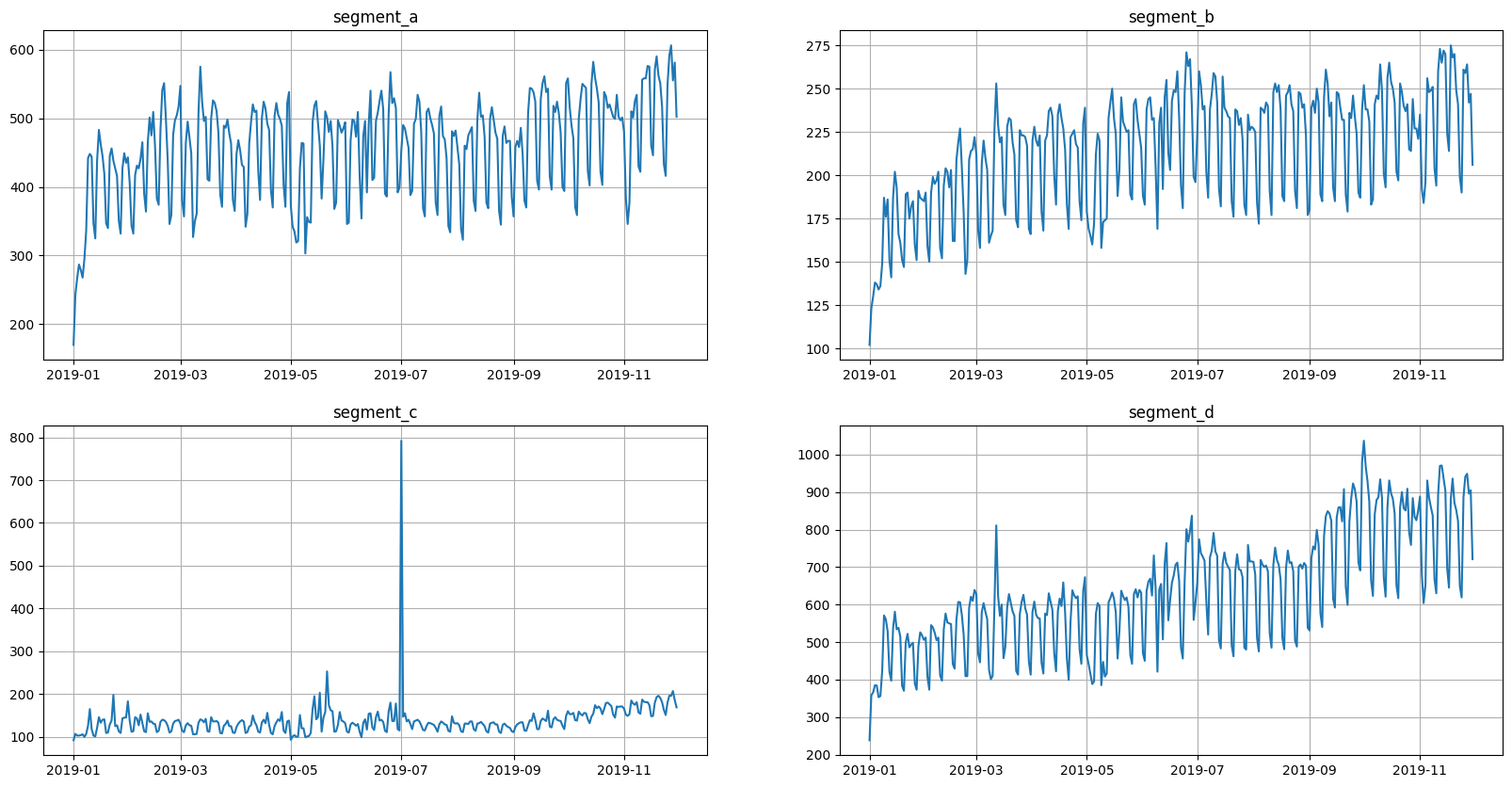
Let’s load and plot the dataset:
[3]:
df = pd.read_csv("data/example_dataset.csv")
df = TSDataset.to_dataset(df)
ts = TSDataset(df, freq="D")

ts.plot()
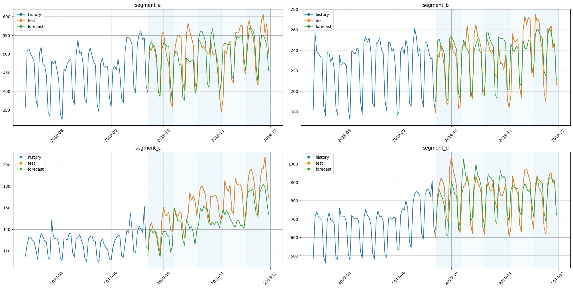
2. Recursive strategy#
Recursive strategy in ETNA is implemented via AutoregressivePipeline.
2.1 AutoRegressivePipeline#
AutoRegressivePipeline is pipeline, which iteratively forecasts step values ahead and after that uses forecasted values to build the features for the next steps.
Could work slowly in case of small
step, since the method needs to recalculate features \(\lceil{\frac{horizon}{step}} \rceil\) timesAllows to use lags, that are lower than
HORIZONCould be imprecise on forecasting with large horizons. The thing is that we accumulate errors of forecasts for further horizons.
Stable for noise-free time series
Note:#
We will add linear trend into the model(because we are working with tree-based models) and use target’s lags as features
[4]:
from etna.pipeline import AutoRegressivePipeline
[5]:
model = CatBoostPerSegmentModel()
transforms = [
    LinearTrendTransform(in_column="target"),
    LagTransform(in_column="target", lags=[i for i in range(1, 1 + NUMBER_OF_LAGS)], out_column="target_lag"),
]

autoregressivepipeline = AutoRegressivePipeline(model=model, transforms=transforms, horizon=HORIZON, step=1)
metrics_recursive_df, forecast_recursive_df, _ = autoregressivepipeline.backtest(
    ts=ts, metrics=[SMAPE(), MAE(), MAPE()]
)
autoregressive_pipeline_metrics = metrics_recursive_df.mean()
[Parallel(n_jobs=1)]: Using backend SequentialBackend with 1 concurrent workers.
[Parallel(n_jobs=1)]: Done   1 out of   1 | elapsed:    7.7s remaining:    0.0s
[Parallel(n_jobs=1)]: Done   2 out of   2 | elapsed:   17.5s remaining:    0.0s
[Parallel(n_jobs=1)]: Done   3 out of   3 | elapsed:   26.9s remaining:    0.0s
[Parallel(n_jobs=1)]: Done   4 out of   4 | elapsed:   35.7s remaining:    0.0s
[Parallel(n_jobs=1)]: Done   5 out of   5 | elapsed:   44.7s remaining:    0.0s
[Parallel(n_jobs=1)]: Done   5 out of   5 | elapsed:   44.7s finished
[6]:
plot_backtest(forecast_recursive_df, ts, history_len=HISTORY_LEN)
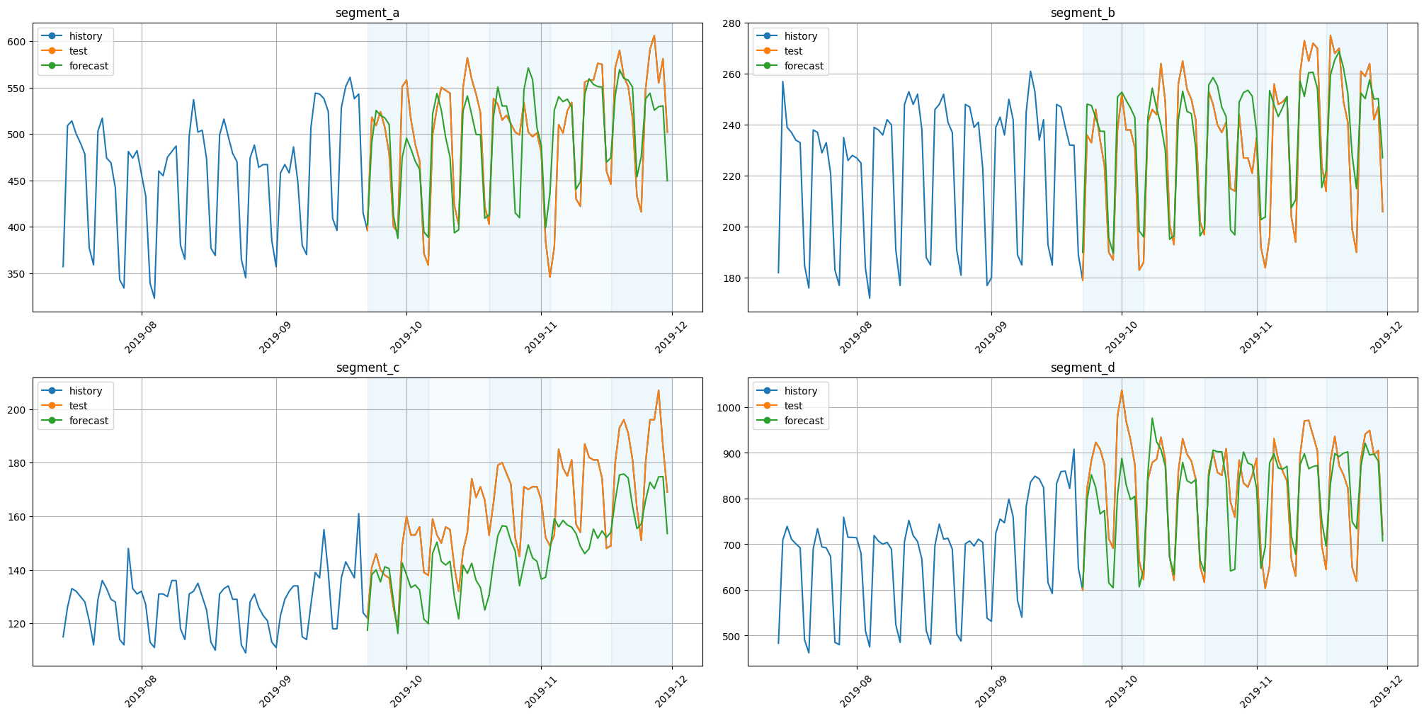
3. Direct Strategy#
Recursive strategy in ETNA is implemented via Pipeline and DirectEnsemble. This strategy assumes conditional independence of forecasts.
3.1 Pipeline#
Pipeline implements the version of direct strategy, where the only one model is fitted to forecast all the points in the future. This implies the several things:
Pipelinedoesn’t accept lags less thanhorizonThis is the most time-efficient method: both in traning and in forecasting
This method might lose the quality with the growth of horizon when using the lags, as the only horizon-far lags are available for all the points
Note:#
As mentioned above, we cannot use lags less than horizon, so now we will use lags from horizon to horizon + number_of_lags
[7]:
from etna.pipeline import Pipeline
[8]:
model = CatBoostPerSegmentModel()
transforms = [
    LinearTrendTransform(in_column="target"),
    LagTransform(in_column="target", lags=list(range(HORIZON, HORIZON + NUMBER_OF_LAGS)), out_column="target_lag"),
]

pipeline = Pipeline(model=model, transforms=transforms, horizon=HORIZON)
metrics_pipeline_df, forecast_pipeline_df, _ = pipeline.backtest(ts=ts, metrics=[SMAPE(), MAE(), MAPE()])
pipeline_metrics = metrics_pipeline_df.mean()
[Parallel(n_jobs=1)]: Using backend SequentialBackend with 1 concurrent workers.
[Parallel(n_jobs=1)]: Done   1 out of   1 | elapsed:    6.1s remaining:    0.0s
[Parallel(n_jobs=1)]: Done   2 out of   2 | elapsed:   14.5s remaining:    0.0s
[Parallel(n_jobs=1)]: Done   3 out of   3 | elapsed:   20.9s remaining:    0.0s
[Parallel(n_jobs=1)]: Done   4 out of   4 | elapsed:   27.1s remaining:    0.0s
[Parallel(n_jobs=1)]: Done   5 out of   5 | elapsed:   33.0s remaining:    0.0s
[Parallel(n_jobs=1)]: Done   5 out of   5 | elapsed:   33.0s finished
[9]:
plot_backtest(forecast_pipeline_df, ts, history_len=HISTORY_LEN)

3.2 DirectEnsemble#
DirectEnsemble fits the separate pipeline to forecast each time subsegment. Forecasting the future, it selects base pipeline with the shortest horizon that covers the timestamp of the current forecasted point. Let’s see an example of choosing a base pipeline for forecasting:

This method can be useful when we have different pipelines, that are effective on different horizons.
The computational time growth with the number of base pipelines.
The forecasts from this strategy might look like a “broken curve”, this happens because they are obtained from the independent models
Let’s build the separate pipeline for each week of interest. The first week will be forecasted using the lags from 7 to 7 + number_of_lags and the second one with lags from horizon to horizon + number_of_lags. We expect that the using of the near lags for the first week might improve the forecast quality
First, let’s build our pipelines:
[10]:
horizons = [7, 14]

model_1 = CatBoostPerSegmentModel()
transforms_1 = [
    LinearTrendTransform(in_column="target"),
    LagTransform(
        in_column="target", lags=[i for i in range(horizons[0], horizons[0] + NUMBER_OF_LAGS)], out_column="target_lag"
    ),
]
pipeline_1 = Pipeline(model=model_1, transforms=transforms_1, horizon=horizons[0])


model_2 = CatBoostPerSegmentModel()
transforms_2 = [
    LinearTrendTransform(in_column="target"),
    LagTransform(
        in_column="target", lags=[i for i in range(horizons[1], horizons[1] + NUMBER_OF_LAGS)], out_column="target_lag"
    ),
]

pipeline_2 = Pipeline(model=model_2, transforms=transforms_2, horizon=horizons[1])
Secondly, we will create ensemble and forecasts:
[11]:
from etna.ensembles import DirectEnsemble
[12]:
ensemble = DirectEnsemble(pipelines=[pipeline_1, pipeline_2])

metrics_ensemble_df, forecast_ensemble_df, _ = ensemble.backtest(ts=ts, metrics=[SMAPE(), MAE(), MAPE()])
ensemble_metrics = metrics_ensemble_df.mean()
[Parallel(n_jobs=1)]: Using backend SequentialBackend with 1 concurrent workers.
[Parallel(n_jobs=1)]: Using backend SequentialBackend with 1 concurrent workers.
[Parallel(n_jobs=1)]: Done   1 out of   1 | elapsed:    5.1s remaining:    0.0s
[Parallel(n_jobs=1)]: Done   2 out of   2 | elapsed:   10.5s remaining:    0.0s
[Parallel(n_jobs=1)]: Done   2 out of   2 | elapsed:   10.5s finished
[Parallel(n_jobs=1)]: Using backend SequentialBackend with 1 concurrent workers.
[Parallel(n_jobs=1)]: Done   1 out of   1 | elapsed:    0.1s remaining:    0.0s
[Parallel(n_jobs=1)]: Done   2 out of   2 | elapsed:    0.3s remaining:    0.0s
[Parallel(n_jobs=1)]: Done   2 out of   2 | elapsed:    0.3s finished
[Parallel(n_jobs=1)]: Done   1 out of   1 | elapsed:   10.8s remaining:    0.0s
[Parallel(n_jobs=1)]: Using backend SequentialBackend with 1 concurrent workers.
[Parallel(n_jobs=1)]: Done   1 out of   1 | elapsed:    5.9s remaining:    0.0s
[Parallel(n_jobs=1)]: Done   2 out of   2 | elapsed:   12.6s remaining:    0.0s
[Parallel(n_jobs=1)]: Done   2 out of   2 | elapsed:   12.6s finished
[Parallel(n_jobs=1)]: Using backend SequentialBackend with 1 concurrent workers.
[Parallel(n_jobs=1)]: Done   1 out of   1 | elapsed:    0.2s remaining:    0.0s
[Parallel(n_jobs=1)]: Done   2 out of   2 | elapsed:    0.3s remaining:    0.0s
[Parallel(n_jobs=1)]: Done   2 out of   2 | elapsed:    0.3s finished
[Parallel(n_jobs=1)]: Done   2 out of   2 | elapsed:   23.7s remaining:    0.0s
[Parallel(n_jobs=1)]: Using backend SequentialBackend with 1 concurrent workers.
[Parallel(n_jobs=1)]: Done   1 out of   1 | elapsed:    6.5s remaining:    0.0s
[Parallel(n_jobs=1)]: Done   2 out of   2 | elapsed:   12.7s remaining:    0.0s
[Parallel(n_jobs=1)]: Done   2 out of   2 | elapsed:   12.7s finished
[Parallel(n_jobs=1)]: Using backend SequentialBackend with 1 concurrent workers.
[Parallel(n_jobs=1)]: Done   1 out of   1 | elapsed:    0.1s remaining:    0.0s
[Parallel(n_jobs=1)]: Done   2 out of   2 | elapsed:    0.3s remaining:    0.0s
[Parallel(n_jobs=1)]: Done   2 out of   2 | elapsed:    0.3s finished
[Parallel(n_jobs=1)]: Done   3 out of   3 | elapsed:   36.8s remaining:    0.0s
[Parallel(n_jobs=1)]: Using backend SequentialBackend with 1 concurrent workers.
[Parallel(n_jobs=1)]: Done   1 out of   1 | elapsed:    6.8s remaining:    0.0s
[Parallel(n_jobs=1)]: Done   2 out of   2 | elapsed:   14.2s remaining:    0.0s
[Parallel(n_jobs=1)]: Done   2 out of   2 | elapsed:   14.2s finished
[Parallel(n_jobs=1)]: Using backend SequentialBackend with 1 concurrent workers.
[Parallel(n_jobs=1)]: Done   1 out of   1 | elapsed:    0.2s remaining:    0.0s
[Parallel(n_jobs=1)]: Done   2 out of   2 | elapsed:    0.3s remaining:    0.0s
[Parallel(n_jobs=1)]: Done   2 out of   2 | elapsed:    0.3s finished
[Parallel(n_jobs=1)]: Done   4 out of   4 | elapsed:   51.3s remaining:    0.0s
[Parallel(n_jobs=1)]: Using backend SequentialBackend with 1 concurrent workers.
[Parallel(n_jobs=1)]: Done   1 out of   1 | elapsed:    7.7s remaining:    0.0s
[Parallel(n_jobs=1)]: Done   2 out of   2 | elapsed:   14.6s remaining:    0.0s
[Parallel(n_jobs=1)]: Done   2 out of   2 | elapsed:   14.6s finished
[Parallel(n_jobs=1)]: Using backend SequentialBackend with 1 concurrent workers.
[Parallel(n_jobs=1)]: Done   1 out of   1 | elapsed:    0.1s remaining:    0.0s
[Parallel(n_jobs=1)]: Done   2 out of   2 | elapsed:    0.3s remaining:    0.0s
[Parallel(n_jobs=1)]: Done   2 out of   2 | elapsed:    0.3s finished
[Parallel(n_jobs=1)]: Done   5 out of   5 | elapsed:  1.1min remaining:    0.0s
[Parallel(n_jobs=1)]: Done   5 out of   5 | elapsed:  1.1min finished
[13]:
plot_backtest(forecast_ensemble_df, ts, history_len=HISTORY_LEN)
3.3 assemble pipelines with DirectEnsemble#
DirectEnsemble described above requires the building of the separate pipeline for each of the time subsegment. This pipelines often has many common parts and differs only in the few places. To make the definition of the pipelines a little bit shorter, you can use assemble_pipelines. It generates the pipelines using the following rules:
Input models(horizons) can be specified as one model(horizon) or as a sequence of models(horizons). In first case all generated pipelines will have input model(horizon) and in the second case
i-th pipeline will holdi-th model(horizon).Transforms can be specified as a sequence of transform or as a sequence of sequences of transforms. Let’s look at some examples to understand better transformations with transforms:
Let’s consider that A, B, C, D, E are different transforms.
Example 1#
If input transform sequence is [A, B, C], function will put [A, B, C] for each pipeline
Example 2#
If input transform sequence is [A, [B, C], D, E], function will put [A, B, D, E] for the first generated pipeline and [A, C, D, E] for the second.
Example 3#
If input transform sequence is [A, [B, C], [D, E]], function will put [A, B, D] for the first generated pipeline and [A, C, E] for the second.
Example 4#
If input transform sequence is [A, [B, None]], function will put [A, B] for the first generated pipeline and [A] for the second.
Let’s build the ensemble from the previous section using assemble_pipelines
[14]:
from etna.pipeline import assemble_pipelines
[15]:
models = [CatBoostPerSegmentModel(), CatBoostPerSegmentModel()]
transforms = [
    LinearTrendTransform(in_column="target"),
    [
        LagTransform(
            in_column="target",
            lags=[i for i in range(horizons[0], horizons[0] + NUMBER_OF_LAGS)],
            out_column="target_lag",
        ),
        LagTransform(
            in_column="target",
            lags=[i for i in range(horizons[1], horizons[1] + NUMBER_OF_LAGS)],
            out_column="target_lag",
        ),
    ],
]

pipelines = assemble_pipelines(models=models, transforms=transforms, horizons=horizons)
pipelines
[15]:
[Pipeline(model = CatBoostPerSegmentModel(iterations = None, depth = None, learning_rate = None, logging_level = 'Silent', l2_leaf_reg = None, thread_count = None, ), transforms = [LinearTrendTransform(in_column = 'target', poly_degree = 1, ), LagTransform(in_column = 'target', lags = [7, 8, 9, 10, 11, 12, 13, 14, 15, 16, 17, 18, 19, 20, 21, 22, 23, 24, 25, 26, 27], out_column = 'target_lag', )], horizon = 7, ),
 Pipeline(model = CatBoostPerSegmentModel(iterations = None, depth = None, learning_rate = None, logging_level = 'Silent', l2_leaf_reg = None, thread_count = None, ), transforms = [LinearTrendTransform(in_column = 'target', poly_degree = 1, ), LagTransform(in_column = 'target', lags = [14, 15, 16, 17, 18, 19, 20, 21, 22, 23, 24, 25, 26, 27, 28, 29, 30, 31, 32, 33, 34], out_column = 'target_lag', )], horizon = 14, )]
Pipelines generation process looks now a bit simpler, isn’t it? Now it’s time to create DirectEnsemble out of them:
[16]:
ensemble = DirectEnsemble(pipelines=pipelines)

metrics_ensemble_df_2, forecast_ensemble_df_2, _ = ensemble.backtest(ts=ts, metrics=[SMAPE(), MAE(), MAPE()])
[Parallel(n_jobs=1)]: Using backend SequentialBackend with 1 concurrent workers.
[Parallel(n_jobs=1)]: Using backend SequentialBackend with 1 concurrent workers.
[Parallel(n_jobs=1)]: Done   1 out of   1 | elapsed:    8.2s remaining:    0.0s
[Parallel(n_jobs=1)]: Done   2 out of   2 | elapsed:   15.5s remaining:    0.0s
[Parallel(n_jobs=1)]: Done   2 out of   2 | elapsed:   15.5s finished
[Parallel(n_jobs=1)]: Using backend SequentialBackend with 1 concurrent workers.
[Parallel(n_jobs=1)]: Done   1 out of   1 | elapsed:    0.1s remaining:    0.0s
[Parallel(n_jobs=1)]: Done   2 out of   2 | elapsed:    0.3s remaining:    0.0s
[Parallel(n_jobs=1)]: Done   2 out of   2 | elapsed:    0.3s finished
[Parallel(n_jobs=1)]: Done   1 out of   1 | elapsed:   15.8s remaining:    0.0s
[Parallel(n_jobs=1)]: Using backend SequentialBackend with 1 concurrent workers.
[Parallel(n_jobs=1)]: Done   1 out of   1 | elapsed:    7.4s remaining:    0.0s
[Parallel(n_jobs=1)]: Done   2 out of   2 | elapsed:   14.7s remaining:    0.0s
[Parallel(n_jobs=1)]: Done   2 out of   2 | elapsed:   14.7s finished
[Parallel(n_jobs=1)]: Using backend SequentialBackend with 1 concurrent workers.
[Parallel(n_jobs=1)]: Done   1 out of   1 | elapsed:    0.1s remaining:    0.0s
[Parallel(n_jobs=1)]: Done   2 out of   2 | elapsed:    0.3s remaining:    0.0s
[Parallel(n_jobs=1)]: Done   2 out of   2 | elapsed:    0.3s finished
[Parallel(n_jobs=1)]: Done   2 out of   2 | elapsed:   30.9s remaining:    0.0s
[Parallel(n_jobs=1)]: Using backend SequentialBackend with 1 concurrent workers.
[Parallel(n_jobs=1)]: Done   1 out of   1 | elapsed:    7.2s remaining:    0.0s
[Parallel(n_jobs=1)]: Done   2 out of   2 | elapsed:   14.3s remaining:    0.0s
[Parallel(n_jobs=1)]: Done   2 out of   2 | elapsed:   14.3s finished
[Parallel(n_jobs=1)]: Using backend SequentialBackend with 1 concurrent workers.
[Parallel(n_jobs=1)]: Done   1 out of   1 | elapsed:    0.1s remaining:    0.0s
[Parallel(n_jobs=1)]: Done   2 out of   2 | elapsed:    0.3s remaining:    0.0s
[Parallel(n_jobs=1)]: Done   2 out of   2 | elapsed:    0.3s finished
[Parallel(n_jobs=1)]: Done   3 out of   3 | elapsed:   45.5s remaining:    0.0s
[Parallel(n_jobs=1)]: Using backend SequentialBackend with 1 concurrent workers.
[Parallel(n_jobs=1)]: Done   1 out of   1 | elapsed:    6.9s remaining:    0.0s
[Parallel(n_jobs=1)]: Done   2 out of   2 | elapsed:   13.8s remaining:    0.0s
[Parallel(n_jobs=1)]: Done   2 out of   2 | elapsed:   13.8s finished
[Parallel(n_jobs=1)]: Using backend SequentialBackend with 1 concurrent workers.
[Parallel(n_jobs=1)]: Done   1 out of   1 | elapsed:    0.1s remaining:    0.0s
[Parallel(n_jobs=1)]: Done   2 out of   2 | elapsed:    0.3s remaining:    0.0s
[Parallel(n_jobs=1)]: Done   2 out of   2 | elapsed:    0.3s finished
[Parallel(n_jobs=1)]: Done   4 out of   4 | elapsed:   59.6s remaining:    0.0s
[Parallel(n_jobs=1)]: Using backend SequentialBackend with 1 concurrent workers.
[Parallel(n_jobs=1)]: Done   1 out of   1 | elapsed:    7.0s remaining:    0.0s
[Parallel(n_jobs=1)]: Done   2 out of   2 | elapsed:   13.6s remaining:    0.0s
[Parallel(n_jobs=1)]: Done   2 out of   2 | elapsed:   13.6s finished
[Parallel(n_jobs=1)]: Using backend SequentialBackend with 1 concurrent workers.
[Parallel(n_jobs=1)]: Done   1 out of   1 | elapsed:    0.1s remaining:    0.0s
[Parallel(n_jobs=1)]: Done   2 out of   2 | elapsed:    0.3s remaining:    0.0s
[Parallel(n_jobs=1)]: Done   2 out of   2 | elapsed:    0.3s finished
[Parallel(n_jobs=1)]: Done   5 out of   5 | elapsed:  1.2min remaining:    0.0s
[Parallel(n_jobs=1)]: Done   5 out of   5 | elapsed:  1.2min finished
Let’s check that the forecasts has not changed:
[17]:
pd.testing.assert_frame_equal(metrics_ensemble_df_2, metrics_ensemble_df)
4.Summary#
In this notebook, we discussed forecasting strategies available in ETNA and look at the examples of their usage. In conclusion, let’s compare their quality on the considered dataset:
[18]:
df_res = pd.DataFrame(
    data=[ensemble_metrics, pipeline_metrics, autoregressive_pipeline_metrics],
    index=["direct_ensemble", "pipeline", "autoregressive_pipeline"],
).drop("fold_number", axis=1)
df_res = df_res.sort_values(by="SMAPE")
df_res
[18]:
| SMAPE | MAE | MAPE | |
|---|---|---|---|
| direct_ensemble | 7.152913 | 28.657613 | 7.004382 |
| autoregressive_pipeline | 7.247425 | 29.945816 | 7.117746 |
| pipeline | 7.319264 | 28.476013 | 7.102676 |