View Jupyter notebook on the GitHub.

Forecast interpretation notebook#

This notebook contains examples of forecast decomposition into additive components for various models.

Table of contents * Forecast decomposition * CatBoost * SARIMAX * BATS * In-sample and out-of-sample decomposition * Accessing target components * Regressors relevance * Feature relevance * Components relevance

[1]:

import warnings

warnings.filterwarnings("ignore")

[2]:

from copy import deepcopy
import pandas as pd

from etna.analysis import plot_backtest
from etna.analysis import plot_forecast_decomposition
from etna.datasets import TSDataset
from etna.pipeline import Pipeline
from etna.transforms import LagTransform
from etna.metrics import MAE

[3]:

HORIZON = 21

Consider the dataset data/example_dataset.csv.

We will use this data to demonstrate how model forecasts can be decomposed down to additive effects in the ETNA library.

Let’s load and plot this data to get a brief idea of how time series look.

[4]:

df = pd.read_csv("data/example_dataset.csv")
df["timestamp"] = pd.to_datetime(df["timestamp"])
df = TSDataset.to_dataset(df)
ts = TSDataset(df, freq="D")

ts.head(5)

[4]:

segment	segment_a	segment_b	segment_c	segment_d
feature	target	target	target	target
timestamp
2019-01-01	170	102	92	238
2019-01-02	243	123	107	358
2019-01-03	267	130	103	366
2019-01-04	287	138	103	385
2019-01-05	279	137	104	384

[5]:

ts.plot()

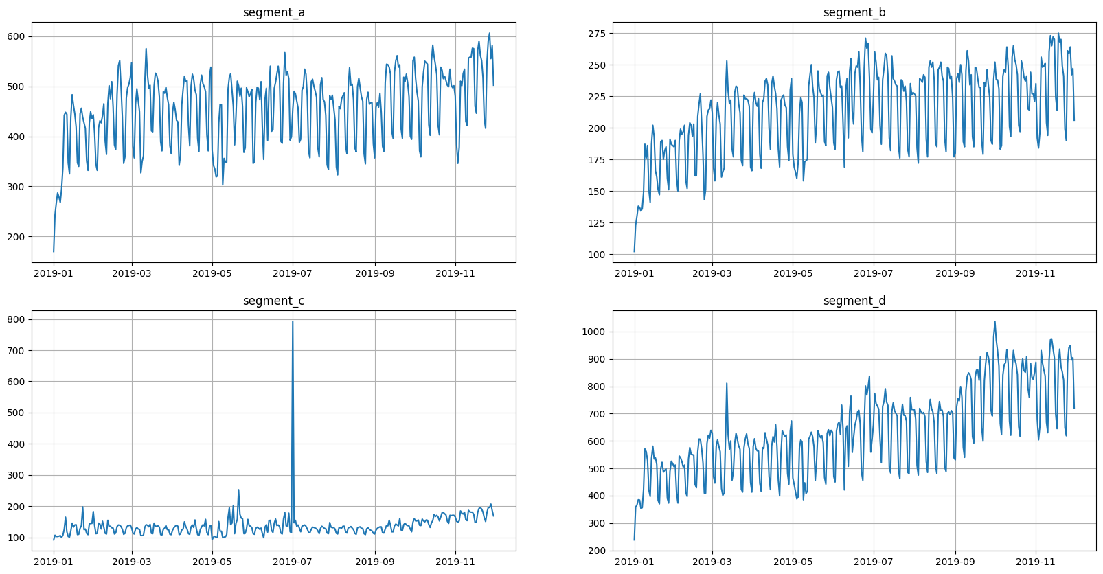
../_images/tutorials_forecast_interpretation_8_0.png

Here we have four segments in the dataset. All segments have seasonalities, and some of them show signs of trend.

Some of the models need features in order to estimate forecasts. Here we will use lags of the target variable as features when it is necessary.

[6]:

transforms = [
    LagTransform(in_column="target", lags=list(range(21, 57, 7)), out_column="lag"),
]

1. Forecast decomposition#

This section shows how a model forecast can be decomposed down to individual additive components. There are two types of decomposition: * model-specific decomposition * model-agnostic decomposition

Model-specific decomposition uses model representation to compute components. Consider linear regression as an example. \(\hat y = w^T X + b\). We can slightly rewrite this equation to see additive components \(\hat y = \sum_{i=0}^m w_i x_i + b\). So in this case, the components are: \(w_i x_i\) and \(b\).

Model-agnostic decomposition uses separate estimators to compute the contribution of each component (e.g., SHAP).

The main feature of forecast decomposition in the ETNA library is guaranteed additive components.

There are several models with available decomposition: * SARIMAXModel * AutoARIMAModel * CatBoostPerSegmentModel, CatBoostMultiSegmentModel * SimpleExpSmoothingModel, HoltModel, HoltWintersModel * LinearPerSegmentModel, ElasticPerSegmentModel, LinearMultiSegmentModel, ElasticMultiSegmentModel * ProphetModel * MovingAverageModel, NaiveModel, DeadlineMovingAverageModel, SeasonalMovingAverageModel * BATS, TBATS

In this notebook, we will take a closer look at the forecast decomposition for CatBoost, SARIMAX and BATS.

Here is a function that will help us extract the target and its components from the forecast dataframe and transform this data to TSDataset.

[7]:

from etna.datasets.utils import match_target_components


def target_components_to_ts(df: pd.DataFrame) -> TSDataset:
    """Get components with target as `TSDataset`."""
    # find target components column names
    column_names = set(df.columns.get_level_values("feature"))
    components_columns = match_target_components(column_names)

    # select dataframe with components
    target_components = df.loc[:, pd.IndexSlice[:, tuple(components_columns)]]

    # select dataframe with target
    target = df.loc[:, pd.IndexSlice[:, "target"]]

    # creat dataset
    forecast_ts = TSDataset(df=target, freq="D")
    forecast_ts.add_target_components(target_components_df=target_components)

    return forecast_ts

1.1 CatBoost#

CatBoost uses model-agnostic forecast decomposition. Components contributions estimated with SHAP for each timestamp. Decomposition at timestamp \(t\) could be represented as:

\begin{equation} f(x_t) = \phi_0 + \sum_{i = 1}^m \phi_i \quad , \end{equation}

where \(\phi_i\) - SHAP values.

[8]:

from etna.models import CatBoostPerSegmentModel
from etna.models import CatBoostMultiSegmentModel

Here we create Pipeline with CatBoostPerSegmentModel and estimate forecast components.

[9]:

pipeline = Pipeline(model=CatBoostPerSegmentModel(), transforms=transforms, horizon=HORIZON)

_, forecast_df, _ = pipeline.backtest(ts=ts, metrics=[MAE()], n_folds=3, forecast_params={"return_components": True})

[Parallel(n_jobs=1)]: Using backend SequentialBackend with 1 concurrent workers.
[Parallel(n_jobs=1)]: Done   1 out of   1 | elapsed:    2.8s remaining:    0.0s
[Parallel(n_jobs=1)]: Done   2 out of   2 | elapsed:    5.9s remaining:    0.0s
[Parallel(n_jobs=1)]: Done   3 out of   3 | elapsed:    8.8s remaining:    0.0s
[Parallel(n_jobs=1)]: Done   3 out of   3 | elapsed:    8.8s finished
[Parallel(n_jobs=1)]: Using backend SequentialBackend with 1 concurrent workers.
[Parallel(n_jobs=1)]: Done   1 out of   1 | elapsed:    0.4s remaining:    0.0s
[Parallel(n_jobs=1)]: Done   2 out of   2 | elapsed:    0.8s remaining:    0.0s
[Parallel(n_jobs=1)]: Done   3 out of   3 | elapsed:    1.2s remaining:    0.0s
[Parallel(n_jobs=1)]: Done   3 out of   3 | elapsed:    1.2s finished
[Parallel(n_jobs=1)]: Using backend SequentialBackend with 1 concurrent workers.
[Parallel(n_jobs=1)]: Done   1 out of   1 | elapsed:    0.0s remaining:    0.0s
[Parallel(n_jobs=1)]: Done   2 out of   2 | elapsed:    0.0s remaining:    0.0s
[Parallel(n_jobs=1)]: Done   3 out of   3 | elapsed:    0.0s remaining:    0.0s
[Parallel(n_jobs=1)]: Done   3 out of   3 | elapsed:    0.0s finished

[10]:

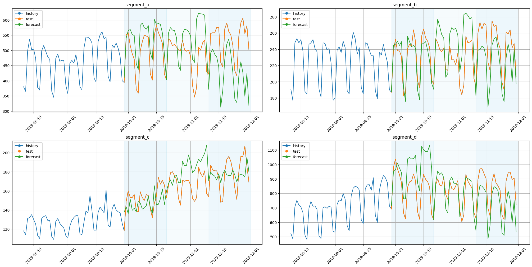
plot_backtest(forecast_df=forecast_df, ts=ts, history_len=50)

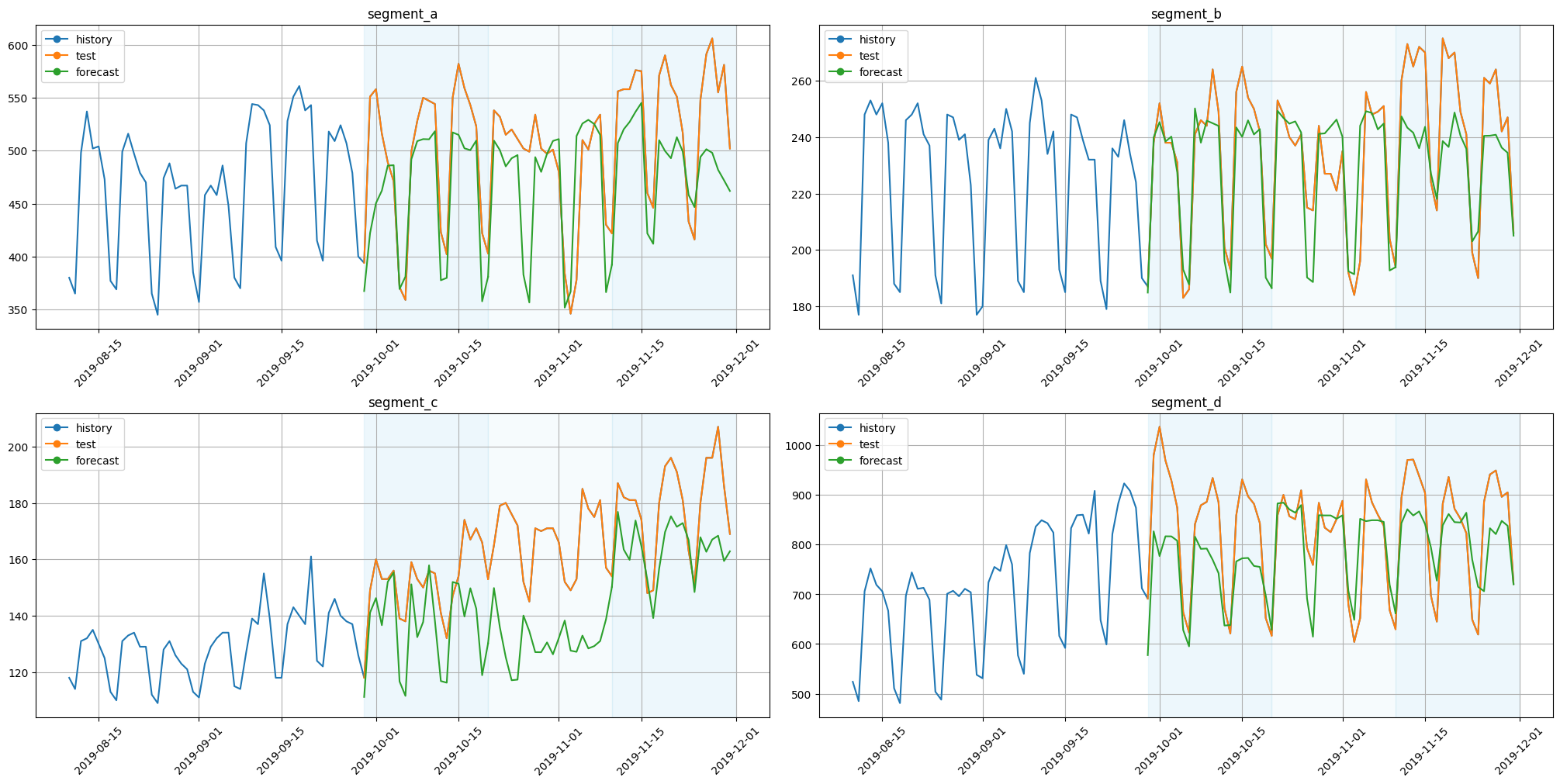
../_images/tutorials_forecast_interpretation_19_0.png

Components could be plotted with the function plot_forecast_decomposition.

[11]:

forecast_ts = target_components_to_ts(df=forecast_df)
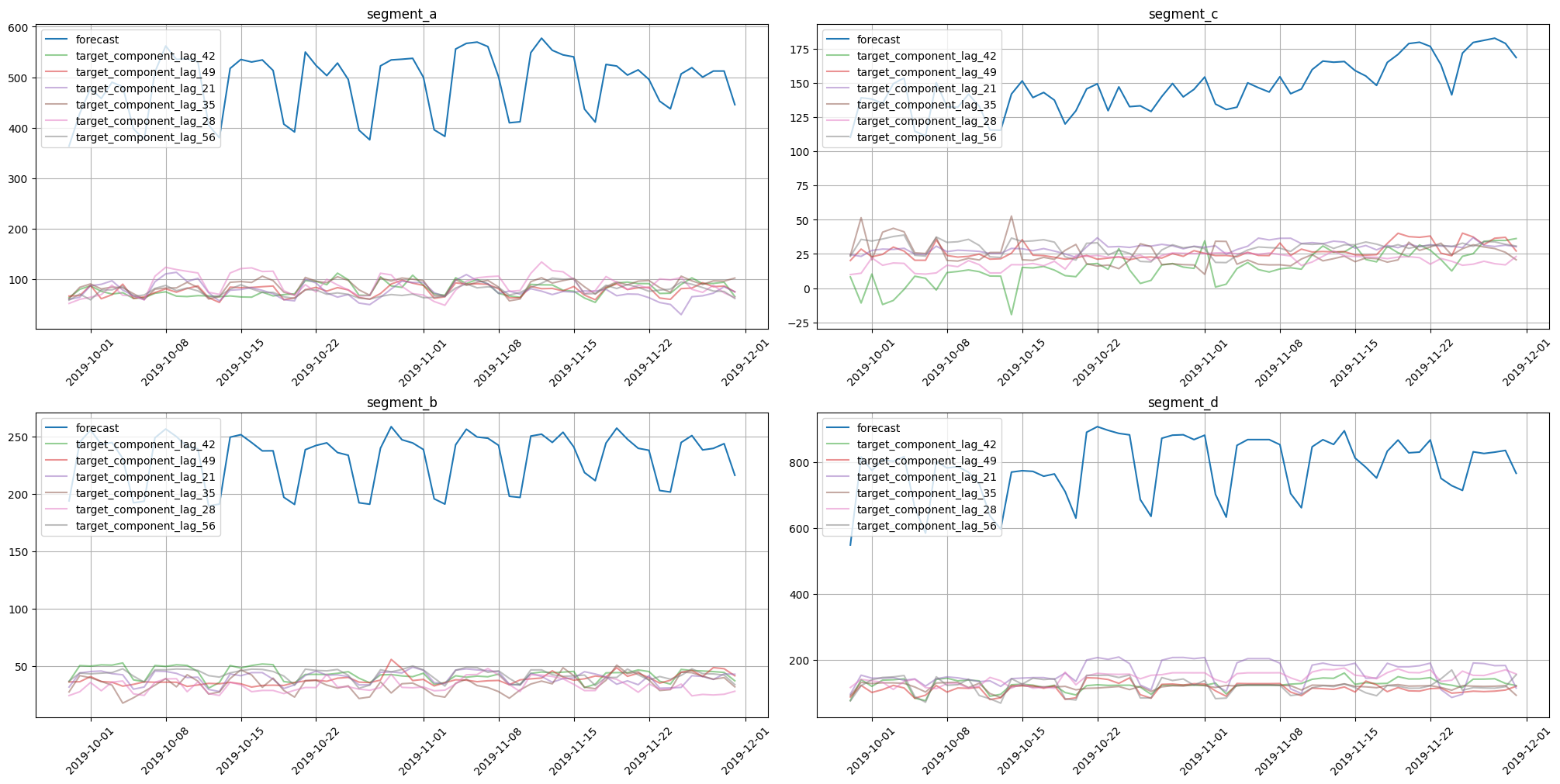
plot_forecast_decomposition(forecast_ts=forecast_ts, mode="joint", columns_num=2, show_grid=True)

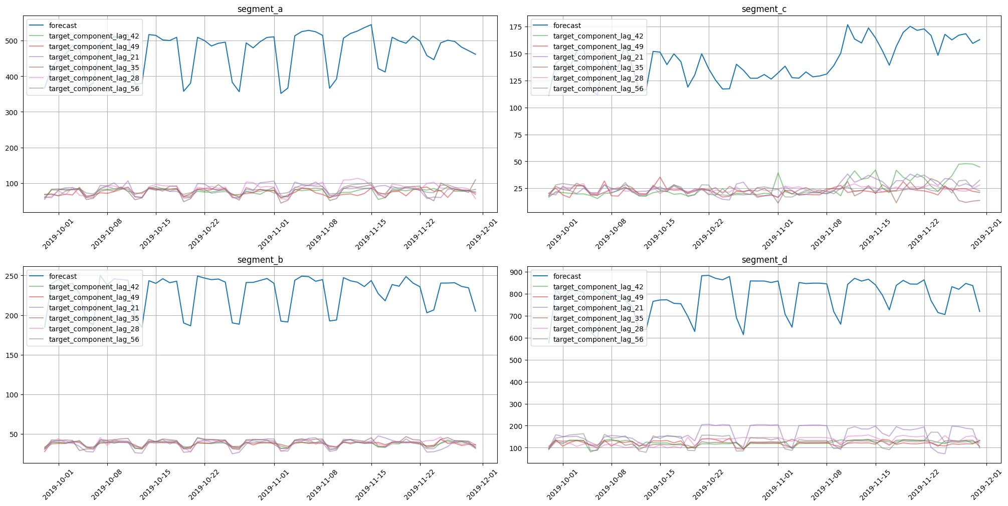
../_images/tutorials_forecast_interpretation_21_0.png

On these charts we can see how each feature contributed to the forecast for each timestamp. CatBoost uses features to estimate forecasts, so each forecast component corresponds to a particular feature.

Let’s run a similar procedure for CatBoostMultiSegmentModel.

[12]:

pipeline = Pipeline(model=CatBoostMultiSegmentModel(), transforms=transforms, horizon=HORIZON)

_, forecast_df, _ = pipeline.backtest(ts=ts, metrics=[MAE()], n_folds=3, forecast_params={"return_components": True})

[Parallel(n_jobs=1)]: Using backend SequentialBackend with 1 concurrent workers.
[Parallel(n_jobs=1)]: Done   1 out of   1 | elapsed:    1.0s remaining:    0.0s
[Parallel(n_jobs=1)]: Done   2 out of   2 | elapsed:    2.2s remaining:    0.0s
[Parallel(n_jobs=1)]: Done   3 out of   3 | elapsed:    3.4s remaining:    0.0s
[Parallel(n_jobs=1)]: Done   3 out of   3 | elapsed:    3.4s finished
[Parallel(n_jobs=1)]: Using backend SequentialBackend with 1 concurrent workers.
[Parallel(n_jobs=1)]: Done   1 out of   1 | elapsed:    0.3s remaining:    0.0s
[Parallel(n_jobs=1)]: Done   2 out of   2 | elapsed:    0.6s remaining:    0.0s
[Parallel(n_jobs=1)]: Done   3 out of   3 | elapsed:    1.0s remaining:    0.0s
[Parallel(n_jobs=1)]: Done   3 out of   3 | elapsed:    1.0s finished
[Parallel(n_jobs=1)]: Using backend SequentialBackend with 1 concurrent workers.
[Parallel(n_jobs=1)]: Done   1 out of   1 | elapsed:    0.0s remaining:    0.0s
[Parallel(n_jobs=1)]: Done   2 out of   2 | elapsed:    0.0s remaining:    0.0s
[Parallel(n_jobs=1)]: Done   3 out of   3 | elapsed:    0.0s remaining:    0.0s
[Parallel(n_jobs=1)]: Done   3 out of   3 | elapsed:    0.0s finished

[13]:

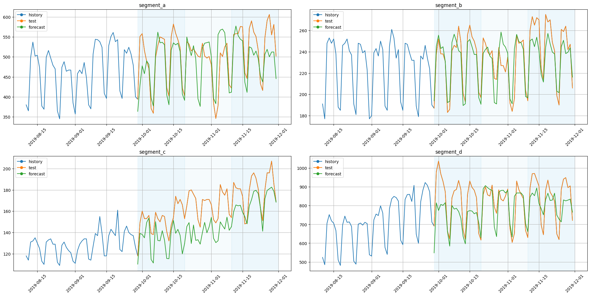
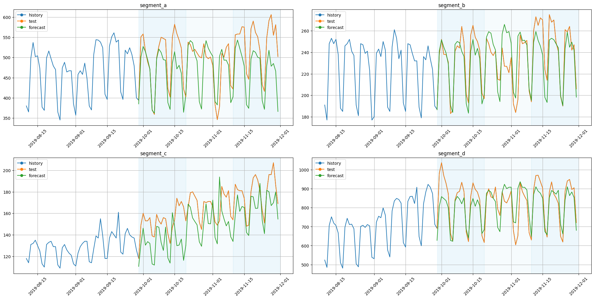
plot_backtest(forecast_df=forecast_df, ts=ts, history_len=50)

../_images/tutorials_forecast_interpretation_25_0.png

[14]:

forecast_ts = target_components_to_ts(df=forecast_df)
plot_forecast_decomposition(forecast_ts=forecast_ts, mode="joint", columns_num=2, show_grid=True)

../_images/tutorials_forecast_interpretation_26_0.png

Here we obtained almost similar results. They are identical in structure but slightly different when comparing values. Such behaviour is explained by the use of a single model for all dataset segments.

1.2 SARIMAX#

SARIMAX uses model-specific forecast decomposition. So the main components of this model are: SARIMA and effects from exogenous variables.

Such constraints on decomposition form are due to implementation details of SARIMAX models, which are estimated as state-space models.

[15]:

from etna.models import SARIMAXModel

Let’s build Pipeline with SARIMAXModel and estimate forecast components on backtest.

[16]:

pipeline = Pipeline(model=SARIMAXModel(), transforms=transforms, horizon=HORIZON)

_, forecast_df, _ = pipeline.backtest(ts=ts, metrics=[MAE()], n_folds=3, forecast_params={"return_components": True})

[Parallel(n_jobs=1)]: Using backend SequentialBackend with 1 concurrent workers.
[Parallel(n_jobs=1)]: Done   1 out of   1 | elapsed:    4.0s remaining:    0.0s
[Parallel(n_jobs=1)]: Done   2 out of   2 | elapsed:    7.5s remaining:    0.0s
[Parallel(n_jobs=1)]: Done   3 out of   3 | elapsed:   12.3s remaining:    0.0s
[Parallel(n_jobs=1)]: Done   3 out of   3 | elapsed:   12.3s finished
[Parallel(n_jobs=1)]: Using backend SequentialBackend with 1 concurrent workers.
[Parallel(n_jobs=1)]: Done   1 out of   1 | elapsed:    0.3s remaining:    0.0s
[Parallel(n_jobs=1)]: Done   2 out of   2 | elapsed:    0.6s remaining:    0.0s
[Parallel(n_jobs=1)]: Done   3 out of   3 | elapsed:    1.0s remaining:    0.0s
[Parallel(n_jobs=1)]: Done   3 out of   3 | elapsed:    1.0s finished
[Parallel(n_jobs=1)]: Using backend SequentialBackend with 1 concurrent workers.
[Parallel(n_jobs=1)]: Done   1 out of   1 | elapsed:    0.0s remaining:    0.0s
[Parallel(n_jobs=1)]: Done   2 out of   2 | elapsed:    0.0s remaining:    0.0s
[Parallel(n_jobs=1)]: Done   3 out of   3 | elapsed:    0.1s remaining:    0.0s
[Parallel(n_jobs=1)]: Done   3 out of   3 | elapsed:    0.1s finished

[17]:

plot_backtest(forecast_df=forecast_df, ts=ts, history_len=50)

../_images/tutorials_forecast_interpretation_32_0.png

[18]:

forecast_ts = target_components_to_ts(df=forecast_df)
plot_forecast_decomposition(forecast_ts=forecast_ts, mode="joint", columns_num=2, show_grid=True)

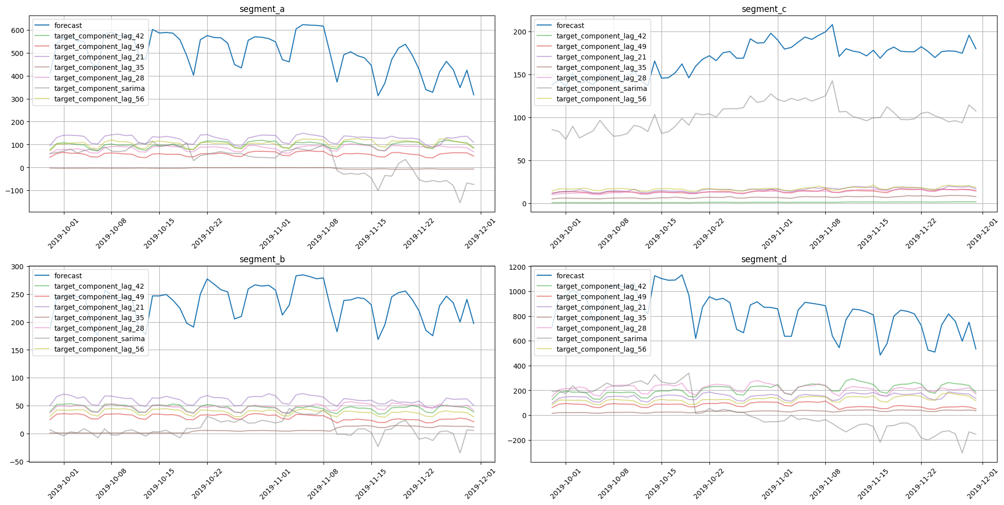
../_images/tutorials_forecast_interpretation_33_0.png

Here we can notice components for each exogenous variable and a separate component for the SARIMA effect. Note that this decomposition is completely different from the forecast decomposition of CatBoost models, even on the same data. This is due to different approaches for component contribution estimation.

1.3 BATS#

BATS uses model-specific forecast decomposition. The main components are: * trend * local level * seasonality for each specified period * errors ARMA(p, q)

The last two components are controlled by seasonal_periods and use_arma_erros parameters, respectively. The trend component is controlled by use_trend. These parameters add flexibility to the model representation and, hence, to the forecast decomposition.

[19]:

from etna.models import BATSModel

Let’s build Pipeline and estimate forecast decomposition with BATSModel, but now without any features.

[20]:

pipeline = Pipeline(model=BATSModel(seasonal_periods=[14, 21]), horizon=HORIZON)

_, forecast_df, _ = pipeline.backtest(ts=ts, metrics=[MAE()], n_folds=3, forecast_params={"return_components": True})

[Parallel(n_jobs=1)]: Using backend SequentialBackend with 1 concurrent workers.
[Parallel(n_jobs=1)]: Done   1 out of   1 | elapsed:  1.8min remaining:    0.0s
[Parallel(n_jobs=1)]: Done   2 out of   2 | elapsed:  4.2min remaining:    0.0s
[Parallel(n_jobs=1)]: Done   3 out of   3 | elapsed:  6.2min remaining:    0.0s
[Parallel(n_jobs=1)]: Done   3 out of   3 | elapsed:  6.2min finished
[Parallel(n_jobs=1)]: Using backend SequentialBackend with 1 concurrent workers.
[Parallel(n_jobs=1)]: Done   1 out of   1 | elapsed:    0.0s remaining:    0.0s
[Parallel(n_jobs=1)]: Done   2 out of   2 | elapsed:    0.1s remaining:    0.0s
[Parallel(n_jobs=1)]: Done   3 out of   3 | elapsed:    0.2s remaining:    0.0s
[Parallel(n_jobs=1)]: Done   3 out of   3 | elapsed:    0.2s finished
[Parallel(n_jobs=1)]: Using backend SequentialBackend with 1 concurrent workers.
[Parallel(n_jobs=1)]: Done   1 out of   1 | elapsed:    0.0s remaining:    0.0s
[Parallel(n_jobs=1)]: Done   2 out of   2 | elapsed:    0.0s remaining:    0.0s
[Parallel(n_jobs=1)]: Done   3 out of   3 | elapsed:    0.0s remaining:    0.0s
[Parallel(n_jobs=1)]: Done   3 out of   3 | elapsed:    0.0s finished

[21]:

plot_backtest(forecast_df=forecast_df, ts=ts, history_len=50)

../_images/tutorials_forecast_interpretation_39_0.png

[22]:

forecast_ts = target_components_to_ts(df=forecast_df)
plot_forecast_decomposition(forecast_ts=forecast_ts, mode="joint", columns_num=2, show_grid=True)

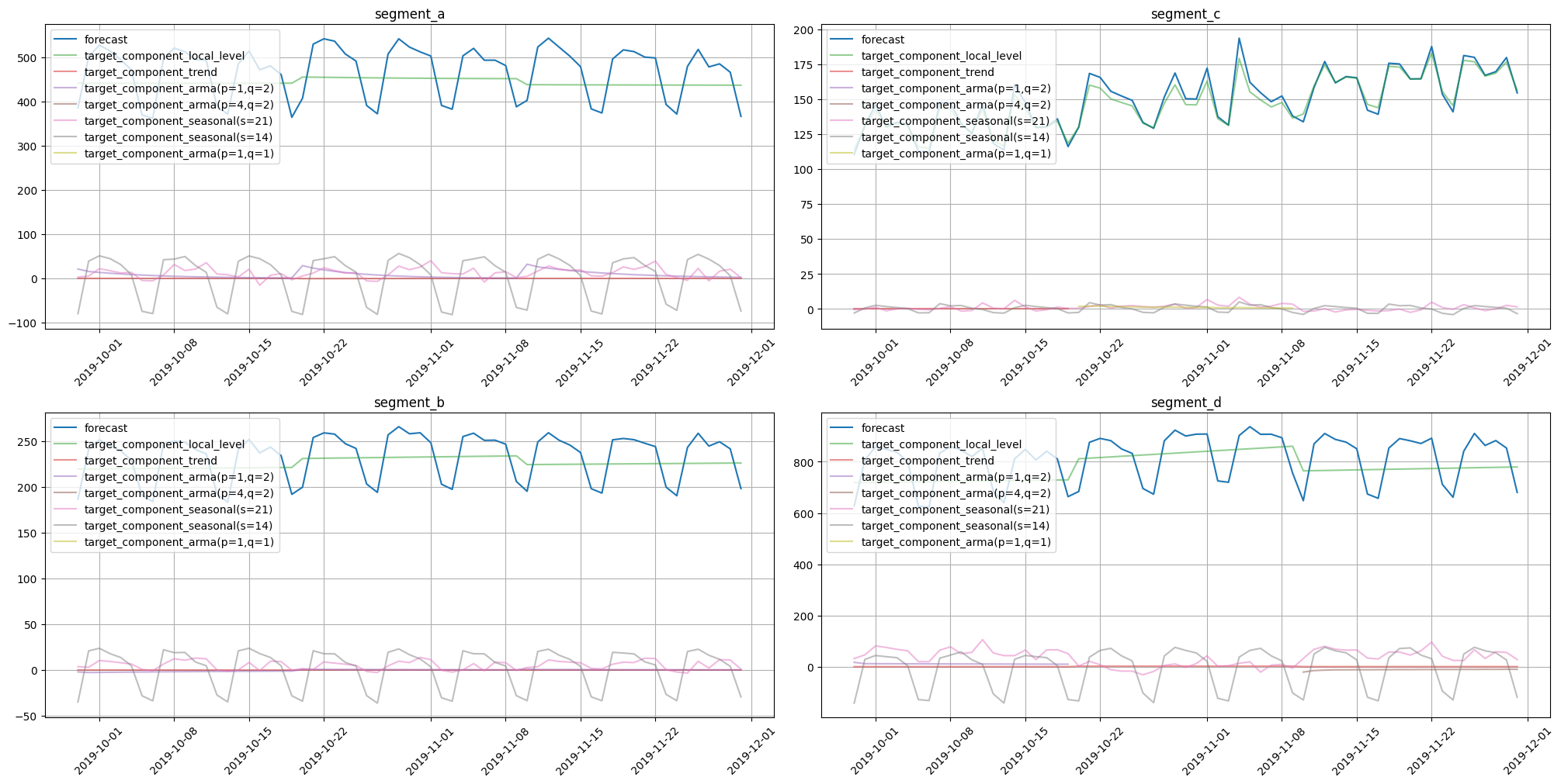
../_images/tutorials_forecast_interpretation_40_0.png

Here we obtained components for trend, local level, seasonality, and ARMA errors. Note that each seasonality period is represented by a separate component. Such a form of decomposition helps to find causality with seasonal effects in the original data. Results show that almost all seasonal fluctuations come from seasonality in period 14.

1.4 In-sample and out-of-sample decomposition#

In the ETNA library we can perform decomposition of fitted and forecasted values separately.

Consider the BATS model with seasonal periods of 2 and 3 weeks. Let’s prepare data for training and forecasting and fit the model.

[23]:

train, _ = ts.train_test_split(test_size=HORIZON)
future = train.make_future(future_steps=HORIZON)

model = BATSModel(seasonal_periods=[14, 21])
model.fit(ts=train);

In-sample forecast decomposition could be estimated with predict method. To do this set return_components=True.

[24]:

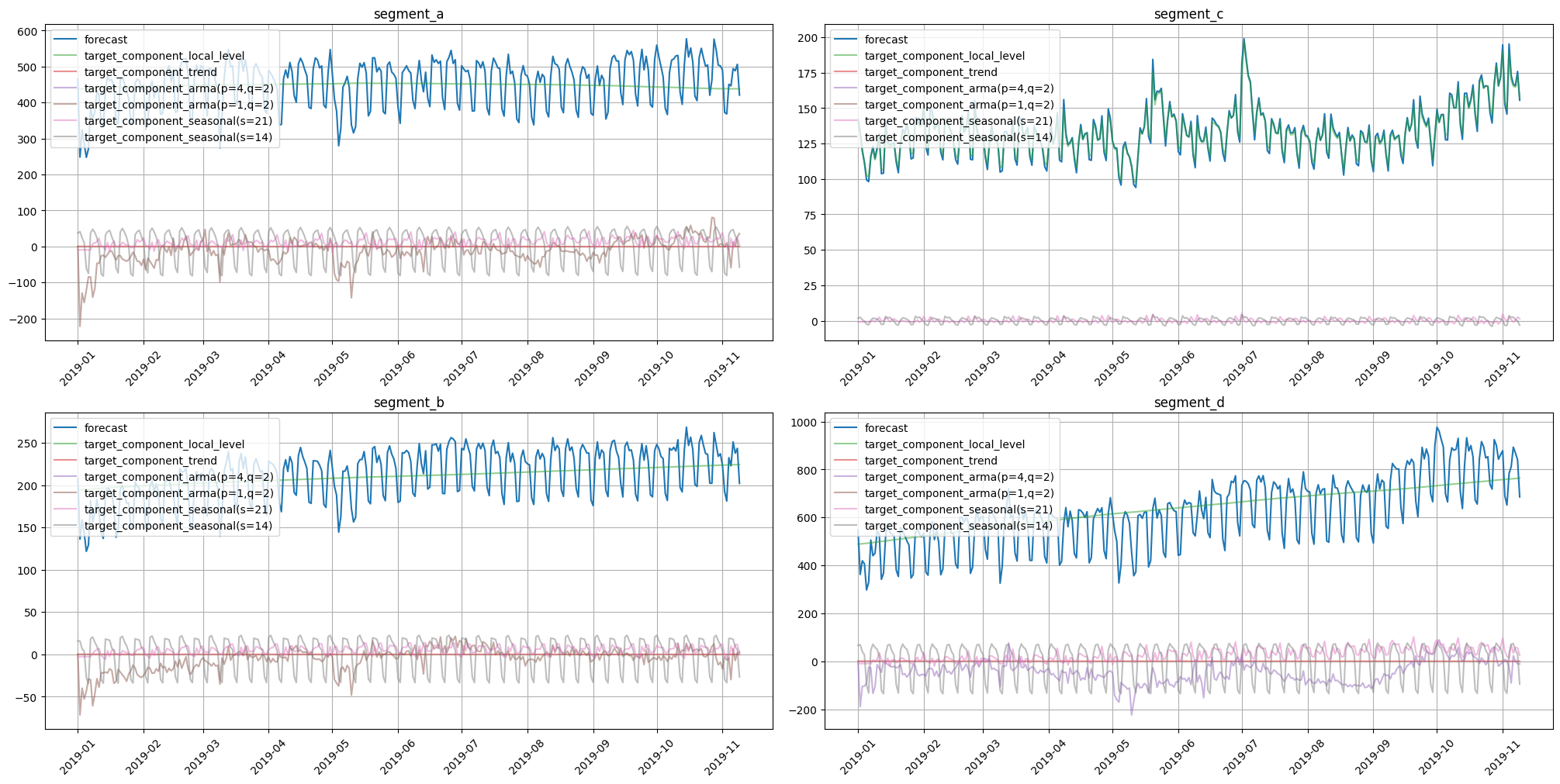
in_sample_forecast = model.predict(ts=train, return_components=True)
plot_forecast_decomposition(forecast_ts=in_sample_forecast, mode="joint", columns_num=2, show_grid=True)

../_images/tutorials_forecast_interpretation_46_0.png

For estimation of out-of-sample forecast decomposition, use forecast with return_components=True.

[25]:

out_of_sample_forecast = model.forecast(ts=future, return_components=True)
plot_forecast_decomposition(forecast_ts=out_of_sample_forecast, mode="joint", columns_num=2, show_grid=True)

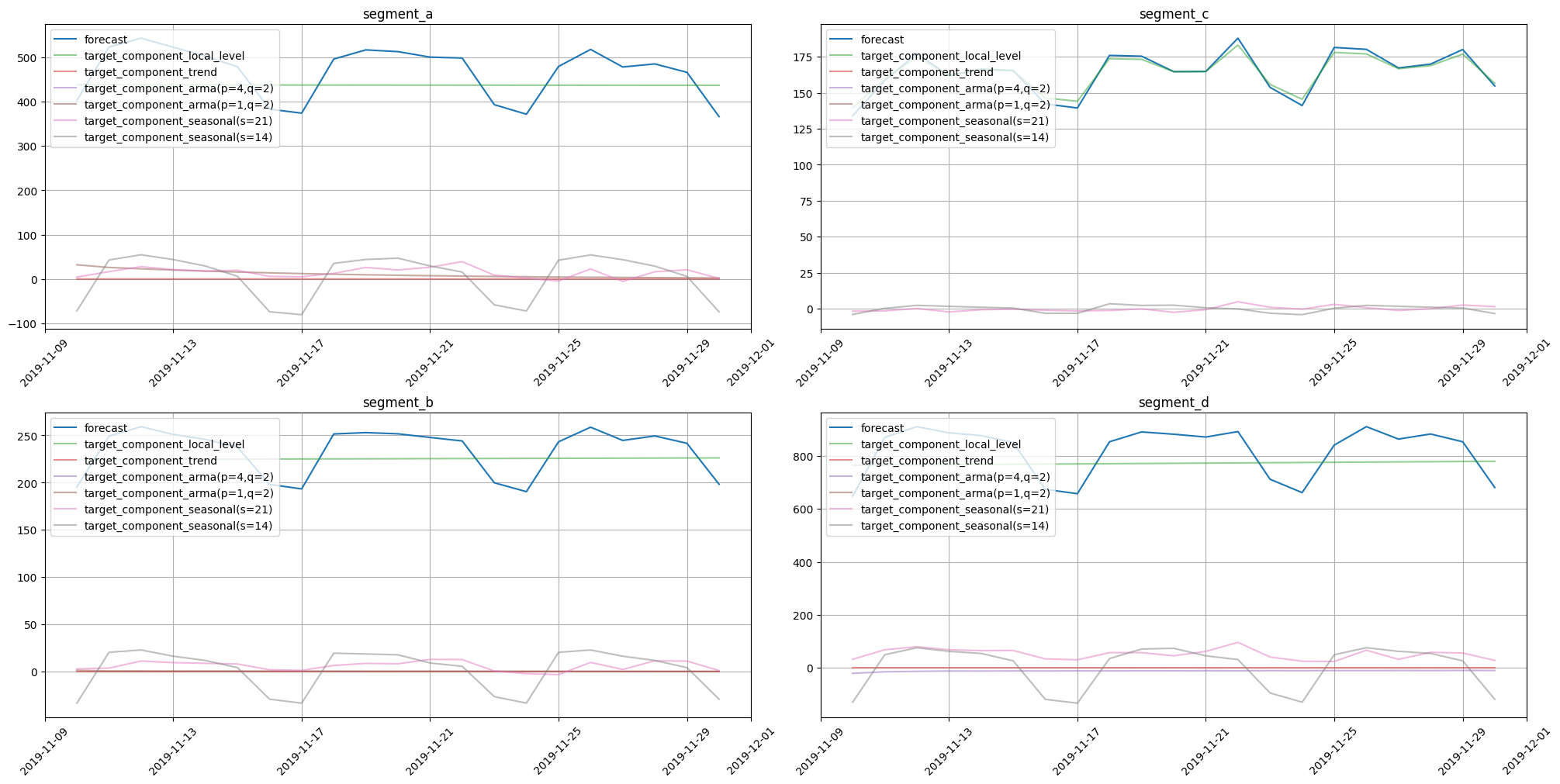
../_images/tutorials_forecast_interpretation_48_0.png

As expected, the decomposition form is the same for in-sample and out-of-sample cases.

2. Accessing target components#

This section shows how one can manipulate forecast components using the TSDataset interface.

Let’s populate our data with lag features and fit the CatBoostPerSegmentModel. We will use this setup to estimate forecast with additive components.

[26]:

ts_with_lags = deepcopy(ts)
ts_with_lags.fit_transform(transforms=transforms)

model = CatBoostPerSegmentModel()
model.fit(ts=ts_with_lags);

Now we can estimate forecasts with forecast decomposition.

[27]:

forecast = model.forecast(ts=ts_with_lags, return_components=True)
forecast

[27]:

segment	segment_a										...	segment_d
feature	lag_21	lag_28	lag_35	lag_42	lag_49	lag_56	target	target_component_lag_21	target_component_lag_28	target_component_lag_35	...	lag_42	lag_49	lag_56	target	target_component_lag_21	target_component_lag_28	target_component_lag_35	target_component_lag_42	target_component_lag_49	target_component_lag_56
timestamp
2019-01-01	NaN	NaN	NaN	NaN	NaN	NaN	368.960244	52.677657	45.848608	59.139714	...	NaN	NaN	NaN	440.294693	58.143024	43.773274	92.546575	76.282320	79.442884	90.106617
2019-01-02	NaN	NaN	NaN	NaN	NaN	NaN	368.960244	52.677657	45.848608	59.139714	...	NaN	NaN	NaN	440.294693	58.143024	43.773274	92.546575	76.282320	79.442884	90.106617
2019-01-03	NaN	NaN	NaN	NaN	NaN	NaN	368.960244	52.677657	45.848608	59.139714	...	NaN	NaN	NaN	440.294693	58.143024	43.773274	92.546575	76.282320	79.442884	90.106617
2019-01-04	NaN	NaN	NaN	NaN	NaN	NaN	368.960244	52.677657	45.848608	59.139714	...	NaN	NaN	NaN	440.294693	58.143024	43.773274	92.546575	76.282320	79.442884	90.106617
2019-01-05	NaN	NaN	NaN	NaN	NaN	NaN	368.960244	52.677657	45.848608	59.139714	...	NaN	NaN	NaN	440.294693	58.143024	43.773274	92.546575	76.282320	79.442884	90.106617
...	...	...	...	...	...	...	...	...	...	...	...	...	...	...	...	...	...	...	...	...	...
2019-11-26	510.0	502.0	532.0	582.0	528.0	558.0	587.562771	92.622123	93.063689	102.406833	...	931.0	879.0	1037.0	937.554113	186.185095	152.507876	144.561146	142.979337	137.269227	174.051432
2019-11-27	501.0	497.0	515.0	559.0	550.0	516.0	602.751237	93.055945	93.196738	98.617847	...	897.0	886.0	969.0	941.766157	189.933535	153.970751	143.035390	142.433922	137.140238	175.252321
2019-11-28	525.0	501.0	520.0	543.0	547.0	489.0	556.927263	89.108979	94.226170	90.372332	...	882.0	934.0	929.0	894.837318	181.561275	154.268641	139.273730	136.903530	130.007170	152.822973
2019-11-29	534.0	480.0	511.0	523.0	544.0	471.0	568.569172	96.026571	92.935954	88.949103	...	843.0	885.0	874.0	899.518552	178.867363	163.091693	144.959843	132.615508	135.207526	144.776619
2019-11-30	430.0	384.0	502.0	422.0	423.0	371.0	499.505858	81.304877	65.772926	113.489016	...	652.0	672.0	664.0	720.744048	108.165250	129.946841	111.854389	124.573300	121.123109	125.081158

334 rows × 52 columns

Note that we have additional columns prefixed with target_component_. These are individual effects that contributed to the overall forecast.

One can obtain forecast components separately from other forecast data using get_target_components.

[28]:

forecast.get_target_components()

[28]:

segment	segment_a						segment_b				...	segment_c				segment_d
feature	target_component_lag_21	target_component_lag_28	target_component_lag_35	target_component_lag_42	target_component_lag_49	target_component_lag_56	target_component_lag_21	target_component_lag_28	target_component_lag_35	target_component_lag_42	...	target_component_lag_35	target_component_lag_42	target_component_lag_49	target_component_lag_56	target_component_lag_21	target_component_lag_28	target_component_lag_35	target_component_lag_42	target_component_lag_49	target_component_lag_56
timestamp
2019-01-01	52.677657	45.848608	59.139714	69.745969	69.187315	72.360981	29.190551	23.342434	27.285093	28.338942	...	18.093097	13.173772	20.646325	19.443199	58.143024	43.773274	92.546575	76.282320	79.442884	90.106617
2019-01-02	52.677657	45.848608	59.139714	69.745969	69.187315	72.360981	29.190551	23.342434	27.285093	28.338942	...	18.093097	13.173772	20.646325	19.443199	58.143024	43.773274	92.546575	76.282320	79.442884	90.106617
2019-01-03	52.677657	45.848608	59.139714	69.745969	69.187315	72.360981	29.190551	23.342434	27.285093	28.338942	...	18.093097	13.173772	20.646325	19.443199	58.143024	43.773274	92.546575	76.282320	79.442884	90.106617
2019-01-04	52.677657	45.848608	59.139714	69.745969	69.187315	72.360981	29.190551	23.342434	27.285093	28.338942	...	18.093097	13.173772	20.646325	19.443199	58.143024	43.773274	92.546575	76.282320	79.442884	90.106617
2019-01-05	52.677657	45.848608	59.139714	69.745969	69.187315	72.360981	29.190551	23.342434	27.285093	28.338942	...	18.093097	13.173772	20.646325	19.443199	58.143024	43.773274	92.546575	76.282320	79.442884	90.106617
...	...	...	...	...	...	...	...	...	...	...	...	...	...	...	...	...	...	...	...	...	...
2019-11-26	92.622123	93.063689	102.406833	115.592269	74.912398	108.965459	39.646473	41.938191	48.057205	42.905137	...	28.693191	44.746001	29.506321	24.909083	186.185095	152.507876	144.561146	142.979337	137.269227	174.051432
2019-11-27	93.055945	93.196738	98.617847	104.375155	114.013395	99.492157	44.803978	42.526073	44.869424	44.210031	...	24.689802	48.773621	28.103322	29.071382	189.933535	153.970751	143.035390	142.433922	137.140238	175.252321
2019-11-28	89.108979	94.226170	90.372332	88.756972	112.596508	81.866302	43.636738	39.279155	41.455011	41.251943	...	25.204180	49.273745	30.080450	29.670928	181.561275	154.268641	139.273730	136.903530	130.007170	152.822973
2019-11-29	96.026571	92.935954	88.949103	89.018761	117.011601	84.627183	41.949065	38.703364	42.617386	40.808739	...	22.174713	48.547700	28.981421	26.047110	178.867363	163.091693	144.959843	132.615508	135.207526	144.776619
2019-11-30	81.304877	65.772926	113.489016	86.668521	78.966691	73.303827	38.118666	33.999578	31.914988	33.683397	...	17.088639	45.224635	22.134809	24.102108	108.165250	129.946841	111.854389	124.573300	121.123109	125.081158

334 rows × 24 columns

There is a possibility to remove components. It can be achieved using drop_target_components. This function will remove components inplace. We can ensure that our forecast dataset no longer has any components by using the target_components_names property.

[29]:

components = forecast.get_target_components()
forecast.drop_target_components()
forecast.target_components_names

[29]:

()

There is a possibility to attach components to the forecast dataset as well. The main constraint on components is that, being attached, they should sum up to the target at each timestamp.

[30]:

forecast.add_target_components(components)
forecast.target_components_names

[30]:

('target_component_lag_21',
 'target_component_lag_28',
 'target_component_lag_35',
 'target_component_lag_42',
 'target_component_lag_49',
 'target_component_lag_56')

3. Regressors relevance#

This section shows how regressors relevance could be estimated.

There are two types of relevance estimation in the ETNA library * statistical, based on tsfresh (StatisticsRelevanceTable) * model based (ModelRelevanceTable)

[31]:

from etna.analysis import plot_feature_relevance
from etna.analysis import StatisticsRelevanceTable
from etna.analysis import ModelRelevanceTable
from sklearn.ensemble import RandomForestRegressor

3.1 Feature relevance#

The first step is to prepare the data. Here, we only need features and estimated forecasts.

[32]:

target_with_features = deepcopy(forecast)
target_with_features.drop_target_components()

Let’s estimate feature relevance using a statistical approach. Results can be shown with the help of the plot_feature_relevance function.

[33]:

plot_feature_relevance(ts=target_with_features, relevance_table=StatisticsRelevanceTable())

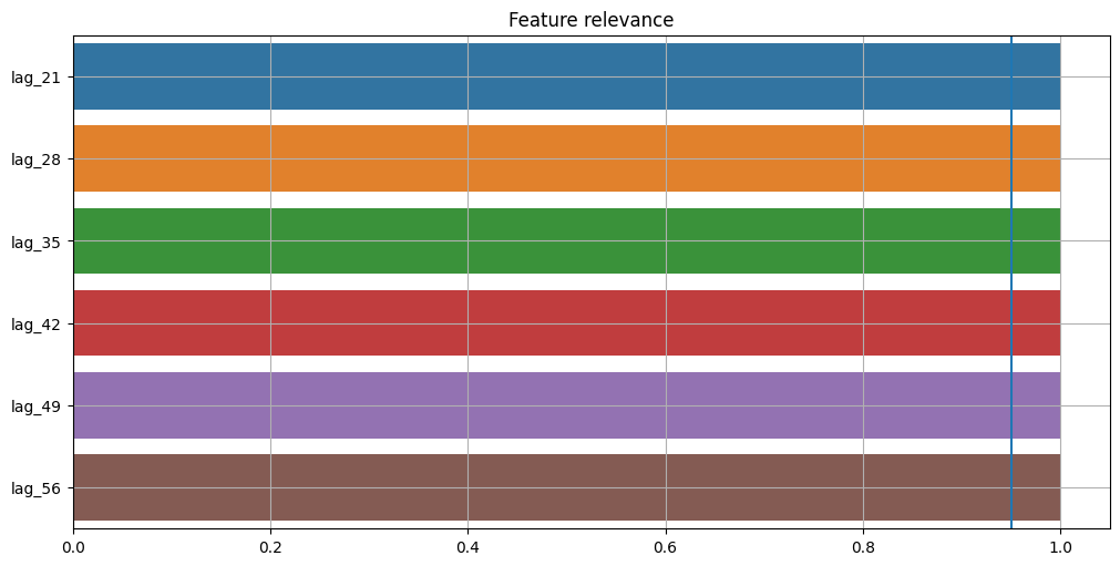
../_images/tutorials_forecast_interpretation_67_0.png

A statistical approach shows that all features have the same relevance. The blue vertical line on the chart represents the significance level. Values that lie to the right of this line have p-value < alpha and values that lie to the left have p-value > alpha. Here we see that all features are significant at the default level of alpha = 0.05. Significance level available only for a statistical approach.

We can use a separate tree-based estimator that is able to provide feature relevance to estimate such values. In this case, we can use RandomForestRegressor.

[34]:

plot_feature_relevance(
    ts=target_with_features,
    relevance_table=ModelRelevanceTable(),
    relevance_params={"model": RandomForestRegressor(random_state=1)},
)

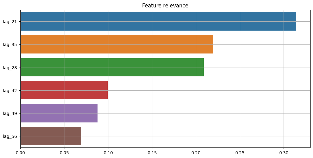
../_images/tutorials_forecast_interpretation_70_0.png

We can see that results from this approach are completely different from statistical results. The main reason is the relevance estimation process. In ModelRelevanceTable, a separate estimator provides feature_importances_, while in StatisticsRelevanceTable statistics from tsfresh are used.

3.2 Components relevance#

We can use the same instruments to estimate relevance for each target component.

First, let’s select only the forecasts with corresponding components from the dataset.

[35]:

target_with_components = TSDataset(df=forecast[:, :, "target"], freq=forecast.freq)
target_components = forecast.get_target_components()
target_with_components.add_target_components(target_components)

Here we can use the same setup with tree-based relevance estimator.

[36]:

plot_feature_relevance(
    ts=target_with_components,
    relevance_table=ModelRelevanceTable(),
    relevance_params={"model": RandomForestRegressor(random_state=1)},
)

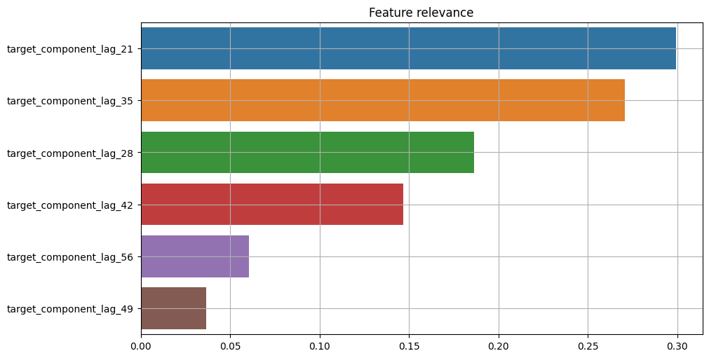
../_images/tutorials_forecast_interpretation_75_0.png

Results show a strong correlation between the relevance of features and the relevance of corresponding components. Note that values are actually different when comparing components to features relevance.

In this notebook we showed how one can decompose in-sample and out-of-sample forecasts in the ETNA library. This decomposition has additive properties and hence may be used for forecast interpretation.

Also, we showed how to estimate regressors relevance with different methods and display the results.